GLM: Poisson Regression
A minimal reproducable example of poisson regression to predict counts using dummy data.
This Notebook is basically an excuse to demo poisson regression using
PyMC3, both manually and using the glm library to demo interactions
using the patsy library. We will create some dummy data, poisson
distributed according to a linear model, and try to recover the
coefficients of that linear model through inference.
For more statistical detail see:
- Basic info on Wikipedia
- GLMs: Poisson regression, exposure, and overdispersion in Chapter 6.2 of ARM, Gelmann & Hill 2006
- This worked example from ARM 6.2 by Clay Ford
This very basic model is insipired by a project by Ian Osvald, which is concerend with understanding the various effects of external environmental factors upon the allergic sneezing of a test subject.
Contents
Package Requirements (shown as a conda-env YAML):
$> less conda_env_pymc3_examples.yml

name: pymc3_examples
channels:
  - defaults
dependencies:
    - python=3.5
    - jupyter
    - ipywidgets
    - numpy
    - scipy
    - matplotlib
    - pandas
    - pytables
    - scikit-learn
    - statsmodels
    - seaborn
    - patsy
    - requests
    - pip
    - pip:
        - regex

$> conda env create --file conda_env_pymc3_examples.yml
$> source activate pymc3_examples
$> pip install --process-dependency-links git+https://github.com/pymc-devs/pymc3
Setup
In [1]:
## Interactive magics
%matplotlib inline
In [2]:
import sys
import warnings
warnings.filterwarnings('ignore')

import re
import numpy as np
import pandas as pd
import matplotlib.pyplot as plt
import seaborn as sns
import patsy as pt
from scipy import optimize

# pymc3 libraries
import pymc3 as pm
import theano as thno
import theano.tensor as T


sns.set(style="darkgrid", palette="muted")
pd.set_option('display.mpl_style', 'default')
plt.rcParams['figure.figsize'] = 14, 6
np.random.seed(0)
Local Functions
In [3]:
def strip_derived_rvs(rvs):
    '''Convenience fn: remove PyMC3-generated RVs from a list'''
    ret_rvs = []
    for rv in rvs:
        if not (re.search('_log',rv.name) or re.search('_interval',rv.name)):
            ret_rvs.append(rv)
    return ret_rvs


def plot_traces_pymc(trcs, varnames=None):
    ''' Convenience fn: plot traces with overlaid means and values '''

    nrows = len(trcs.varnames)
    if varnames is not None:
        nrows = len(varnames)

    ax = pm.traceplot(trcs, varnames=varnames, figsize=(12,nrows*1.4),
                      lines={k: v['mean'] for k, v in
                             pm.df_summary(trcs,varnames=varnames).iterrows()})

    for i, mn in enumerate(pm.df_summary(trcs, varnames=varnames)['mean']):
        ax[i,0].annotate('{:.2f}'.format(mn), xy=(mn,0), xycoords='data',
                         xytext=(5,10), textcoords='offset points', rotation=90,
                         va='bottom', fontsize='large', color='#AA0022')
Generate Data
This dummy dataset is created to emulate some data created as part of a study into quantified self, and the real data is more complicated than this. Ask Ian Osvald if you’d like to know more https://twitter.com/ianozsvald
Assumptions:
- The subject sneezes N times per day, recorded as
nsneeze (int) - The subject may or may not drink alcohol during that day, recorded as
alcohol (boolean) - The subject may or may not take an antihistamine medication during
that day, recorded as the negative action
nomeds (boolean) - I postulate (probably incorrectly) that sneezing occurs at some baseline rate, which increases if an antihistamine is not taken, and further increased after alcohol is consumed.
- The data is aggegated per day, to yield a total count of sneezes on that day, with a boolean flag for alcohol and antihistamine usage, with the big assumption that nsneezes have a direct causal relationship.
Create 4000 days of data: daily counts of sneezes which are poisson distributed w.r.t alcohol consumption and antihistamine usage
In [4]:
# decide poisson theta values
theta_noalcohol_meds = 1    # no alcohol, took an antihist
theta_alcohol_meds = 3      # alcohol, took an antihist
theta_noalcohol_nomeds = 6  # no alcohol, no antihist
theta_alcohol_nomeds = 36   # alcohol, no antihist

# create samples
q = 1000
df = pd.DataFrame({
        'nsneeze': np.concatenate((np.random.poisson(theta_noalcohol_meds, q),
                                   np.random.poisson(theta_alcohol_meds, q),
                                   np.random.poisson(theta_noalcohol_nomeds, q),
                                   np.random.poisson(theta_alcohol_nomeds, q))),
        'alcohol': np.concatenate((np.repeat(False, q),
                                   np.repeat(True, q),
                                   np.repeat(False, q),
                                   np.repeat(True, q))),
        'nomeds': np.concatenate((np.repeat(False, q),
                                      np.repeat(False, q),
                                      np.repeat(True, q),
                                      np.repeat(True, q)))})
In [5]:
df.tail()
Out[5]:
| alcohol | nomeds | nsneeze | |
|---|---|---|---|
| 3995 | True | True | 38 |
| 3996 | True | True | 31 |
| 3997 | True | True | 30 |
| 3998 | True | True | 34 |
| 3999 | True | True | 36 |
View means of the various combinations (poisson mean values)
In [6]:
df.groupby(['alcohol','nomeds']).mean().unstack()
Out[6]:
| nsneeze | ||
|---|---|---|
| nomeds | False | True |
| alcohol | ||
| False | 1.018 | 5.866 |
| True | 2.938 | 35.889 |
Briefly Describe Dataset
In [7]:
g = sns.factorplot(x='nsneeze', row='nomeds', col='alcohol', data=df,
               kind='count', size=4, aspect=1.5)
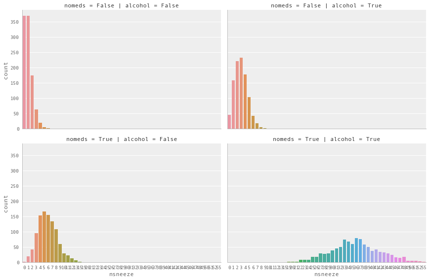
Observe:
- This looks a lot like poisson-distributed count data (because it is)
- With
nomeds == Falseandalcohol == False(top-left, akak antihistamines WERE used, alcohol was NOT drunk) the mean of the poisson distribution of sneeze counts is low. - Changing
alcohol == True(top-right) increases the sneeze countnsneezeslightly - Changing
nomeds == True(lower-left) increases the sneeze countnsneezefurther - Changing both
alcohol == True and nomeds == True(lower-right) increases the sneeze countnsneezea lot, increasing both the mean and variance.
Poisson Regression
Our model here is a very simple Poisson regression, allowing for interaction of terms:
Create linear model for interaction of terms
In [8]:
fml = 'nsneeze ~ alcohol + antihist + alcohol:antihist' # full patsy formulation
In [9]:
fml = 'nsneeze ~ alcohol * nomeds' # lazy, alternative patsy formulation
1. Manual method, create design matrices and manually specify model
Create Design Matrices
In [10]:
(mx_en, mx_ex) = pt.dmatrices(fml, df, return_type='dataframe', NA_action='raise')
In [11]:
pd.concat((mx_ex.head(3),mx_ex.tail(3)))
Out[11]:
| Intercept | alcohol[T.True] | nomeds[T.True] | alcohol[T.True]:nomeds[T.True] | |
|---|---|---|---|---|
| 0 | 1.0 | 0.0 | 0.0 | 0.0 |
| 1 | 1.0 | 0.0 | 0.0 | 0.0 |
| 2 | 1.0 | 0.0 | 0.0 | 0.0 |
| 3997 | 1.0 | 1.0 | 1.0 | 1.0 |
| 3998 | 1.0 | 1.0 | 1.0 | 1.0 |
| 3999 | 1.0 | 1.0 | 1.0 | 1.0 |
Create Model
In [12]:
with pm.Model() as mdl_fish:

    # define priors, weakly informative Normal
    b0 = pm.Normal('b0_intercept', mu=0, sd=10)
    b1 = pm.Normal('b1_alcohol[T.True]', mu=0, sd=10)
    b2 = pm.Normal('b2_nomeds[T.True]', mu=0, sd=10)
    b3 = pm.Normal('b3_alcohol[T.True]:nomeds[T.True]', mu=0, sd=10)

    # define linear model and exp link function
    theta = (b0 +
            b1 * mx_ex['alcohol[T.True]'] +
            b2 * mx_ex['nomeds[T.True]'] +
            b3 * mx_ex['alcohol[T.True]:nomeds[T.True]'])

    ## Define Poisson likelihood
    y = pm.Poisson('y', mu=np.exp(theta), observed=mx_en['nsneeze'].values)
Sample Model
In [13]:
with mdl_fish:
    trc_fish = pm.sample(2000, tune=1000, njobs=4)[1000:]
Auto-assigning NUTS sampler...
Initializing NUTS using ADVI...
Average Loss = 8,741.9:  17%|█▋        | 33556/200000 [00:07<00:37, 4436.96it/s]
Convergence archived at 34000
Interrupted at 34,000 [17%]: Average Loss = 12,493
100%|██████████| 2000/2000 [00:53<00:00, 37.07it/s]
View Diagnostics
In [14]:
rvs_fish = [rv.name for rv in strip_derived_rvs(mdl_fish.unobserved_RVs)]
plot_traces_pymc(trc_fish, varnames=rvs_fish)
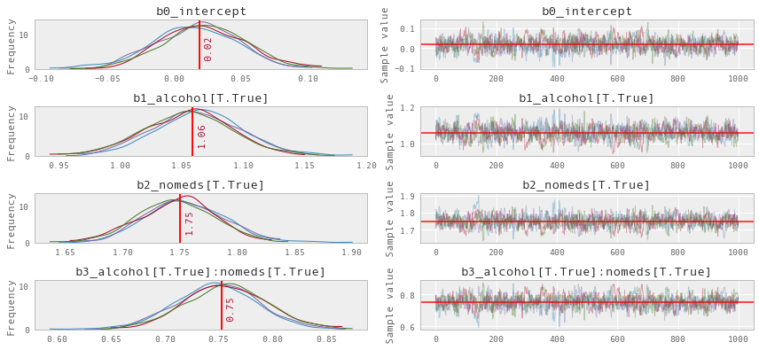
Observe:
- The model converges quickly and traceplots looks pretty well mixed
Transform coeffs and recover theta values
In [15]:
np.exp(pm.df_summary(trc_fish, varnames=rvs_fish)[['mean','hpd_2.5','hpd_97.5']])
Out[15]:
| mean | hpd_2.5 | hpd_97.5 | |
|---|---|---|---|
| b0_intercept | 1.019115 | 0.960588 | 1.084479 |
| b1_alcohol[T.True] | 2.883167 | 2.677978 | 3.083394 |
| b2_nomeds[T.True] | 5.755584 | 5.404332 | 6.166625 |
| b3_alcohol[T.True]:nomeds[T.True] | 2.122313 | 1.960857 | 2.285519 |
Observe:
The contributions from each feature as a multiplier of the baseline sneezecount appear to be as per the data generation:
exp(b0_intercept): mean=1.02 cr=[0.96, 1.08]
Roughly linear baseline count when no alcohol and meds, as per the generated data:
theta_noalcohol_meds = 1 (as set above) theta_noalcohol_meds = exp(b0_intercept) = 1
exp(b1_alcohol): mean=2.88 cr=[2.69, 3.09]
non-zero positive effect of adding alcohol, a ~3x multiplier of baseline sneeze count, as per the generated data:
theta_alcohol_meds = 3 (as set above) theta_alcohol_meds = exp(b0_intercept + b1_alcohol) = exp(b0_intercept) * exp(b1_alcohol) = 1 * 3 = 3
exp(b2_nomeds[T.True]): mean=5.76 cr=[5.40, 6.17]
larger, non-zero positive effect of adding nomeds, a ~6x multiplier of baseline sneeze count, as per the generated data:
theta_noalcohol_nomeds = 6 (as set above) theta_noalcohol_nomeds = exp(b0_intercept + b2_nomeds) = exp(b0_intercept) * exp(b2_nomeds) = 1 * 6 = 6
exp(b3_alcohol[T.True]:nomeds[T.True]): mean=2.12 cr=[1.98, 2.30]
small, positive interaction effect of alcohol and meds, a ~2x multiplier of baseline sneeze count, as per the generated data:
theta_alcohol_nomeds = 36 (as set above) theta_alcohol_nomeds = exp(b0_intercept + b1_alcohol + b2_nomeds + b3_alcohol:nomeds) = exp(b0_intercept) * exp(b1_alcohol) * exp(b2_nomeds * b3_alcohol:nomeds) = 1 * 3 * 6 * 2 = 36
2. Alternative method, using pymc.glm
Create Model
Alternative automatic formulation using ``pmyc.glm``
In [16]:
with pm.Model() as mdl_fish_alt:

    pm.glm.GLM.from_formula(fml, df, family=pm.glm.families.Poisson())
Sample Model
In [17]:
with mdl_fish_alt:
    trc_fish_alt = pm.sample(4000, tune=2000)[2000:]
Auto-assigning NUTS sampler...
Initializing NUTS using ADVI...
Average Loss = 8,752.5:  36%|███▋      | 72995/200000 [00:28<00:48, 2645.19it/s]
Convergence archived at 73000
Interrupted at 73,000 [36%]: Average Loss = 10,558
100%|██████████| 4000/4000 [00:59<00:00, 67.09it/s]
View Traces
In [18]:
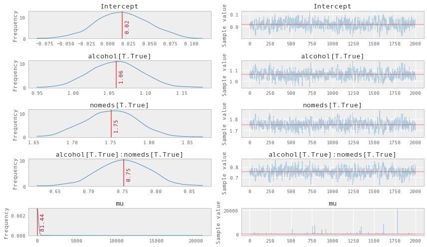
rvs_fish_alt = [rv.name for rv in strip_derived_rvs(mdl_fish_alt.unobserved_RVs)]
plot_traces_pymc(trc_fish_alt, varnames=rvs_fish_alt)
Transform coeffs
In [19]:
np.exp(pm.df_summary(trc_fish_alt, varnames=rvs_fish_alt)[['mean','hpd_2.5','hpd_97.5']])
Out[19]:
| mean | hpd_2.5 | hpd_97.5 | |
|---|---|---|---|
| Intercept | 1.018166e+00 | 0.958267 | 1.081268e+00 |
| alcohol[T.True] | 2.884562e+00 | 2.695548 | 3.099807e+00 |
| nomeds[T.True] | 5.757993e+00 | 5.398246 | 6.140422e+00 |
| alcohol[T.True]:nomeds[T.True] | 2.122279e+00 | 1.972142 | 2.298126e+00 |
| mu | 2.328724e+35 | 1.002232 | 8.016059e+66 |
Observe:
- The traceplots look well mixed
- The transformed model coeffs look moreorless the same as those generated by the manual model
- Note also that the
mucoeff is for the overall mean of the dataset and has an extreme skew, if we look at the median value ...
In [20]:
np.percentile(trc_fish_alt['mu'], [25,50,75])
Out[20]:
array([ 4.04931927, 9.77667856, 23.27432728])
... of 9.45 with a range [25%, 75%] of [4.17, 24.18], we see this is pretty close to the overall mean of:
In [21]:
df['nsneeze'].mean()
Out[21]:
11.42775
Example originally contributed by Jonathan Sedar 2016-05-15 github.com/jonsedar