Kernels / Covariance functions
The following are a series of examples covering each available covariance function, and demonstrating allowed operations. The API will be familiar to users of GPy or GPflow, though ours is simplified. All covariance function parameters can be assigned prior distributions or hardcoded. MCMC methods or optimization methods can be used for inference.
In [4]:
import matplotlib.pyplot as plt
import matplotlib.cm as cmap
%matplotlib inline

import numpy as np
np.random.seed(206)
import theano
import theano.tensor as tt
import pymc3 as pm
In [5]:
X = np.linspace(0,2,200)[:,None]
# function to display covariance matrices
def plot_cov(X, K, stationary=True):
K = K + 1e-8*np.eye(X.shape[0])
x = X.flatten()
fig = plt.figure(figsize=(14,5))
ax1 = fig.add_subplot(121)
m = ax1.imshow(K, cmap="inferno",
interpolation='none',
extent=(np.min(X), np.max(X), np.max(X), np.min(X)));
plt.colorbar(m);
ax1.set_title("Covariance Matrix")
ax1.set_xlabel("X")
ax1.set_ylabel("X")
ax2 = fig.add_subplot(122)
if not stationary:
ax2.plot(x, np.diag(K), "k", lw=2, alpha=0.8)
ax2.set_title("The Diagonal of K")
ax2.set_ylabel("k(x,x)")
else:
ax2.plot(x, K[:,0], "k", lw=2, alpha=0.8)
ax2.set_title("K as a function of x - x'")
ax2.set_ylabel("k(x,x')")
ax2.set_xlabel("X")
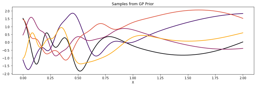
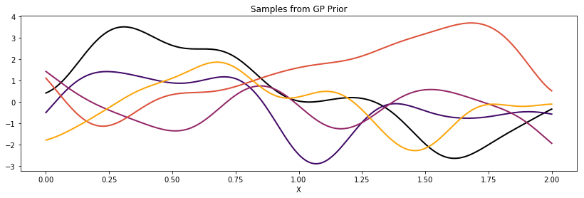
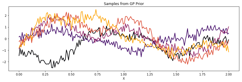
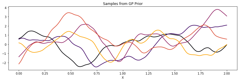
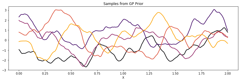
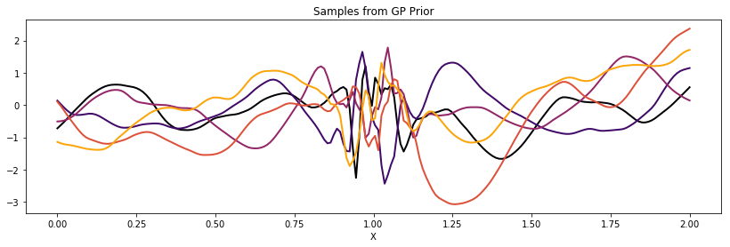
fig = plt.figure(figsize=(14,4))
ax = fig.add_subplot(111)
samples = np.random.multivariate_normal(np.zeros(200), K, 5).T;
for i in range(samples.shape[1]):
ax.plot(x, samples[:,i], color=cmap.inferno(i*0.2), lw=2);
ax.set_title("Samples from GP Prior")
ax.set_xlabel("X")
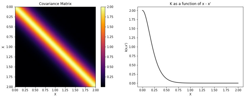
Exponentiated Quadratic
The lengthscale \(l\), overall scaling \(\tau\), and constant bias term \(b\) can be scalars or PyMC3 random variables.
In [6]:
with pm.Model() as model:
    l = 0.2
    tau = 2.0
    b = 0.5
    cov = b + tau * pm.gp.cov.ExpQuad(1, l)

K = theano.function([], cov(X))()
plot_cov(X, K)

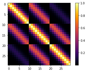
Two (and higher) Dimensional Inputs
Both dimensions active
It is easy to define kernels with higher dimensional inputs. Notice that
the lengthscales parameter is an array of length 2. Lists of PyMC3
random variables can be used for automatic relevance determination
(ARD).
In [7]:
x1, x2 = np.meshgrid(np.linspace(0,1,10), np.arange(1,4))
X2 = np.concatenate((x1.reshape((30,1)), x2.reshape((30,1))), axis=1)

with pm.Model() as model:
    l = np.array([0.2, 1.0])
    cov = pm.gp.cov.ExpQuad(input_dim=2, lengthscales=l)
K = theano.function([], cov(X2))()
m = plt.imshow(K, cmap="inferno", interpolation='none'); plt.colorbar(m);
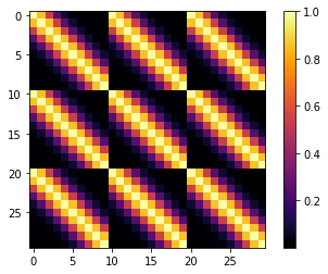
One dimension active
In [8]:
with pm.Model() as model:
    l = 0.2
    cov = pm.gp.cov.ExpQuad(input_dim=2, lengthscales=l,
                            active_dims=[True, False])
K = theano.function([], cov(X2))()
m = plt.imshow(K, cmap="inferno", interpolation='none'); plt.colorbar(m);
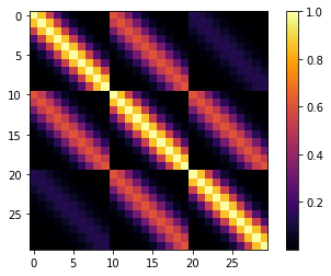
Product of two covariances, active over each dimension
In [9]:
with pm.Model() as model:
    l1 = 0.2
    l2 = 1.0
    cov1 = pm.gp.cov.ExpQuad(2, l1, active_dims=[True, False])
    cov2 = pm.gp.cov.ExpQuad(2, l2, active_dims=[False, True])
    cov = cov1 * cov2
K = theano.function([], cov(X2))()
m = plt.imshow(K, cmap="inferno", interpolation='none'); plt.colorbar(m);
White Noise
In our design, there is no need for a white noise kernel. This case can be handled with Theano. The following is a covariance function that is 5% white noise.
In [10]:
with pm.Model() as model:
    l = 0.2
    sigma2 = 0.05
    tau = 0.95
    cov_latent = tau * pm.gp.cov.ExpQuad(1, l)
    cov_noise = sigma2 * tt.eye(200)

K = theano.function([], cov_latent(X) + cov_noise)()
plot_cov(X, K)

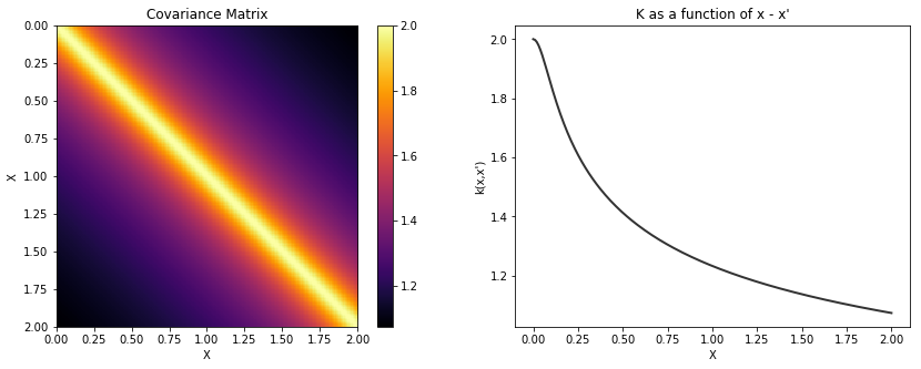
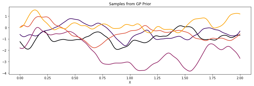
Rational Quadratic
In [11]:
with pm.Model() as model:
    alpha = 0.1
    l = 0.2
    tau = 2.0
    cov = tau * pm.gp.cov.RatQuad(1, l, alpha)

K = theano.function([], cov(X))()

plot_cov(X, K)
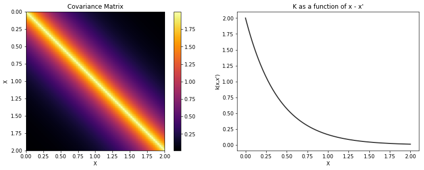
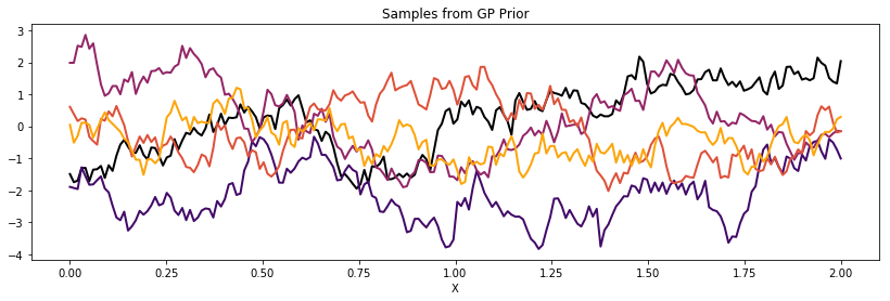
Exponential
In [12]:
with pm.Model() as model:
    l = 0.2
    tau = 2.0
    cov = tau * pm.gp.cov.Exponential(1, l)

K = theano.function([], cov(X))()

plot_cov(X, K)
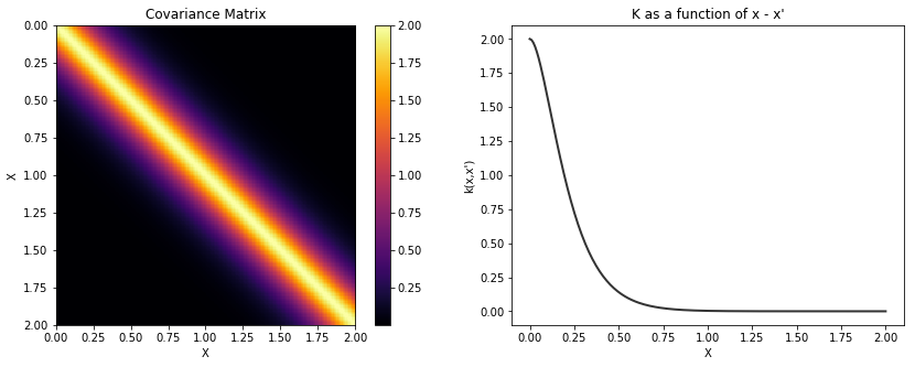
Matern 5/2
In [13]:
with pm.Model() as model:
    l = 0.2
    tau = 2.0
    cov = tau * pm.gp.cov.Matern52(1, l)

K = theano.function([], cov(X))()

plot_cov(X, K)
Matern 3/2
In [14]:
with pm.Model() as model:
    l = 0.2
    tau = 2.0
    cov = tau * pm.gp.cov.Matern32(1, l)

K = theano.function([], cov(X))()

plot_cov(X, K)
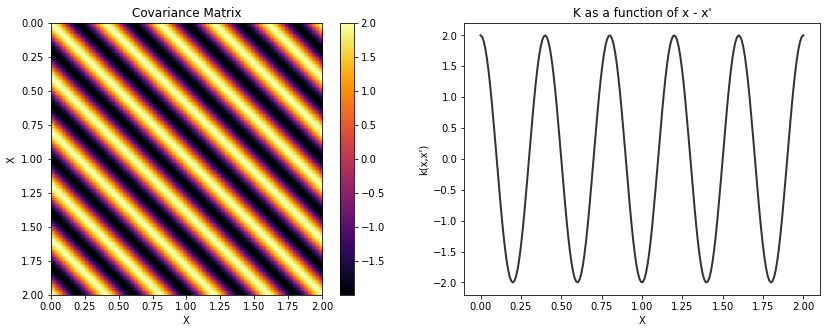
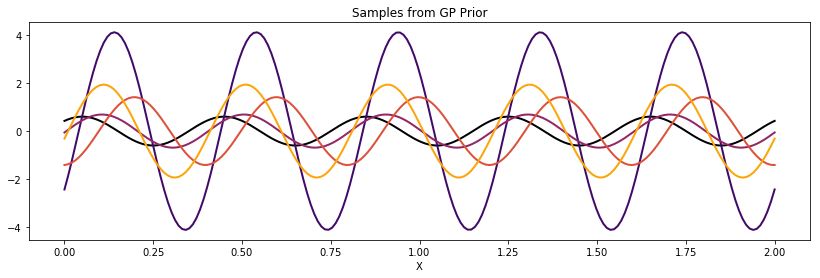
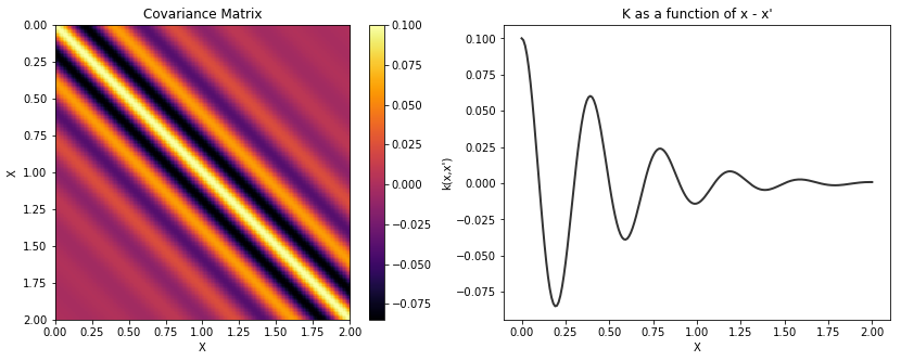
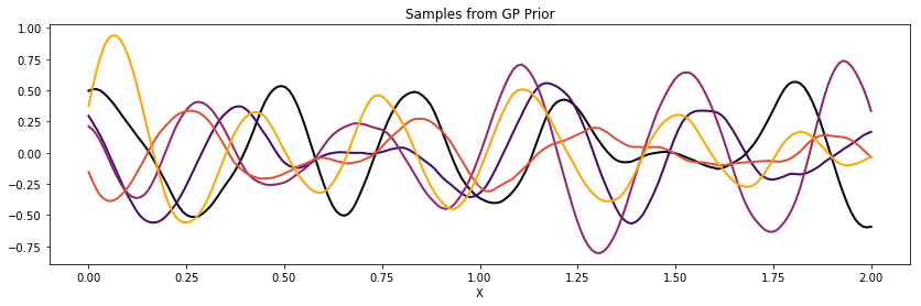
Cosine
In [15]:
with pm.Model() as model:
    l = 0.2
    tau = 2.0
    cov = tau * pm.gp.cov.Cosine(1, l)

K = theano.function([], cov(X))()

plot_cov(X, K)
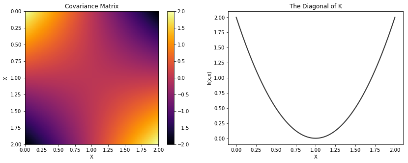
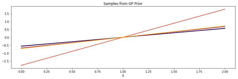
Linear
In [16]:
with pm.Model() as model:
    c = 1.0
    tau = 2.0
    cov = tau * pm.gp.cov.Linear(1, c)

K = theano.function([], cov(X))()

plot_cov(X, K, False)
Polynomial
In [17]:
with pm.Model() as model:
    c = 1.0
    d = 3
    offset = 1.0
    tau = 0.1
    cov = tau * pm.gp.cov.Polynomial(1, c=c, d=d, offset=offset)

K = theano.function([], cov(X))()

plot_cov(X, K, False)
Multiplication with a precomputed covariance matrix
A covariance function cov can be multiplied with numpy matrix,
K_cos.
In [18]:
with pm.Model() as model:
    l = 0.2
    cov_cos = pm.gp.cov.Cosine(1, l)
K_cos = theano.function([], cov_cos(X))()


with pm.Model() as model:
    cov = tau * pm.gp.cov.Matern32(1, 0.5) * K_cos

K = theano.function([], cov(X))()
plot_cov(X, K)
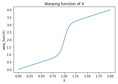
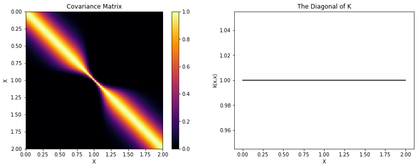
Applying an arbitary warping function on the inputs
If \(k(x, x')\) is a valid covariance function, then so is \(k(w(x), w(x'))\).
The first argument of the warping function must be the input X. The
remaining arguments can be anything else, including (thanks to Theano’s
symbolic differentiation) random variables.
In [19]:
def warp_func(x, a, b, c):
    return 1.0 + x + (a * tt.tanh(b * (x - c)))

with pm.Model() as model:
    a = 1.0
    b = 10.0
    c = 1.0

    cov_m52 = pm.gp.cov.Matern52(1, l)
    cov = pm.gp.cov.WarpedInput(1, warp_func=warp_func, args=(a,b,c), cov_func=cov_m52)

wf = theano.function([], warp_func(X.flatten(), a,b,c))()
plt.plot(X, wf); plt.xlabel("X"); plt.ylabel("warp_func(X)"); plt.title("Warping function of X");

K = theano.function([], cov(X))()
plot_cov(X, K, False)
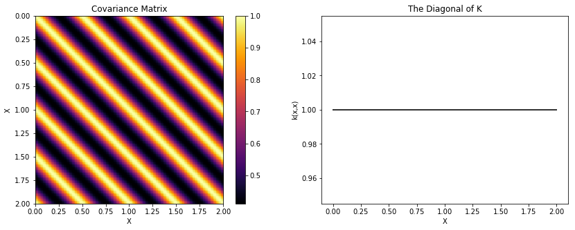
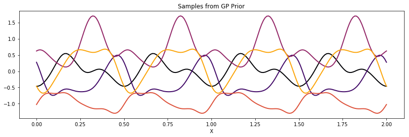
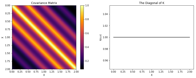
Periodic
The WarpedInput kernel can be used to create the Periodic
covariance. This covariance models functions that are periodic, but are
not an exact sine wave (like the Cosine kernel is).
The periodic kernel is given by
Where T is the period, and \(\ell\) is the lengthscale. It can be
derived by warping the input of an ExpQuad kernel with the function
\(\mathbf{u}(x) = (\sin(2\pi x \frac{1}{T})\,, \cos(2 \pi x \frac{1}{T}))\).
Here we use the WarpedInput kernel to construct it.
The input X, which is defined at the top of this page, is 2
“seconds” long. We use a period of \(0.5\), which means that
functions drawn from this GP prior will repeat 4 times over 2 seconds.
In [27]:
def mapping(x, T):
    c = 2.0 * np.pi * (1.0 / T)
    u = tt.concatenate((tt.sin(c*x), tt.cos(c*x)), 1)
    return u

with pm.Model() as model:
    T = 0.5
    l = 1.5
    # note that the input of the covariance function taking
    #    the inputs is 2 dimensional
    cov_exp = pm.gp.cov.ExpQuad(2, l)
    cov = pm.gp.cov.WarpedInput(1, cov_func=cov_exp,
                                   warp_func=mapping,
                                   args=(T, ))
K = theano.function([], cov(X))()
plot_cov(X, K, False)
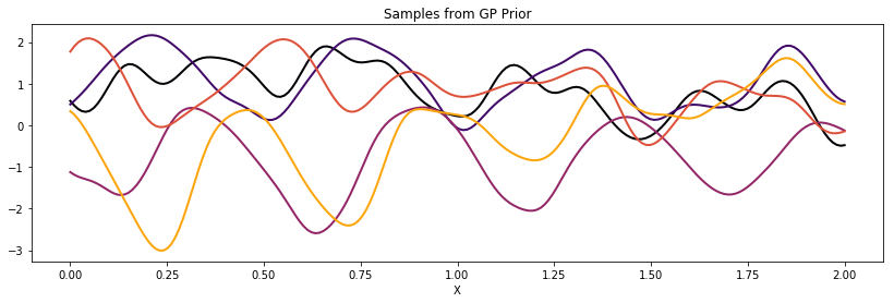
Locally Periodic (Gabor)
Similarly, we can construct a locally periodic, or Gabor, covariance function by multiplying our periodic kernel with a different stationary covariance function.
In [30]:
with pm.Model() as model:
    T = 0.5
    l = 1.5
    l_local = 1.0
    cov_exp = pm.gp.cov.ExpQuad(2, l)
    cov_per = pm.gp.cov.WarpedInput(1, cov_func=cov_exp,
                                       warp_func=mapping,
                                       args=(T, ))
    cov = cov_per * pm.gp.cov.Matern52(1, l_local)
K = theano.function([], cov(X))()
plot_cov(X, K, False)
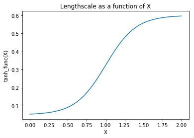
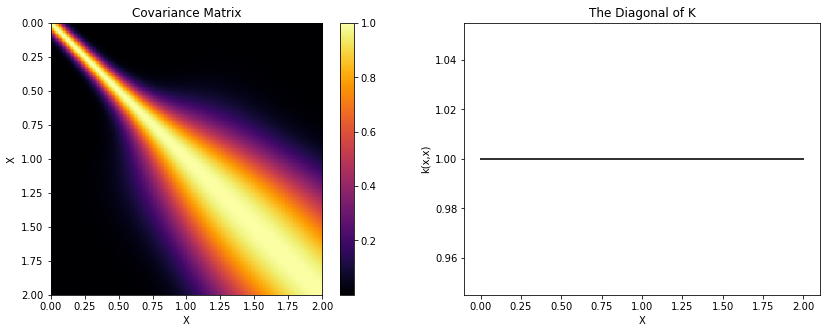
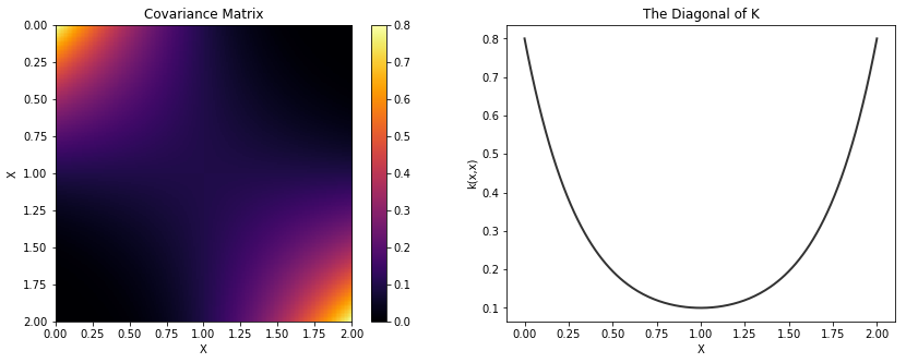
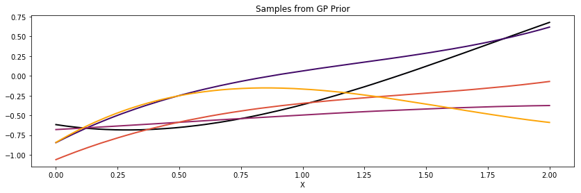
Gibbs
The Gibbs covariance function applies a positive definite warping
function to the lengthscale. Similarly to WarpedInput, the
lengthscale warping function can be specified with parameters that are
either fixed or random variables.
In [31]:
def tanh_func(x, x1, x2, w, x0):
    """
    l1: Left saturation value
    l2: Right saturation value
    lw: Transition width
    x0: Transition location.
    """
    return (x1 + x2) / 2.0 - (x1 - x2) / 2.0 * tt.tanh((x - x0) / w)

with pm.Model() as model:
    l1 = 0.05
    l2 = 0.6
    lw = 0.4
    x0 = 1.0
    cov = pm.gp.cov.Gibbs(1, tanh_func, args=(l1, l2, lw, x0))

wf = theano.function([], tanh_func(X, l1, l2, lw, x0))()
plt.plot(X, wf); plt.ylabel("tanh_func(X)"); plt.xlabel("X"); plt.title("Lengthscale as a function of X");

K = theano.function([], cov(X))()
plot_cov(X, K, False)