Marginalized Gaussian Mixture Model

Author: Austin Rochford

%matplotlib inline

from matplotlib import pyplot as plt
import numpy as np
import pymc3 as pm
import seaborn as sns

SEED = 383561

np.random.seed(SEED) # from random.org, for reproducibility

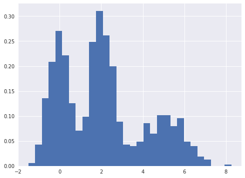
Gaussian mixtures are a flexible class of models for data that exhibits subpopulation heterogeneity. A toy example of such a data set is shown below.

N = 1000

W = np.array([0.35, 0.4, 0.25])

MU = np.array([0., 2., 5.])
SIGMA = np.array([0.5, 0.5, 1.])

component = np.random.choice(MU.size, size=N, p=W)
x = np.random.normal(MU[component], SIGMA[component], size=N)

fig, ax = plt.subplots(figsize=(8, 6))

ax.hist(x, bins=30, normed=True, lw=0);

/opt/conda/lib/python3.5/site-packages/matplotlib/font_manager.py:1297: UserWarning: findfont: Font family ['sans-serif'] not found. Falling back to DejaVu Sans
  (prop.get_family(), self.defaultFamily[fontext]))

A natural parameterization of the Gaussian mixture model is as the latent variable model

\[\begin{split}\begin{align*} \mu_1, \ldots, \mu_K & \sim N(0, \sigma^2) \\ \tau_1, \ldots, \tau_K & \sim \textrm{Gamma}(a, b) \\ \boldsymbol{w} & \sim \textrm{Dir}(\boldsymbol{\alpha}) \\ z\ |\ \boldsymbol{w} & \sim \textrm{Cat}(\boldsymbol{w}) \\ x\ |\ z & \sim N(\mu_z, \tau^{-1}_z). \end{align*}\end{split}\]

An implementation of this parameterization in PyMC3 is available here. A drawback of this parameterization is that is posterior relies on sampling the discrete latent variable \(z\). This reliance can cause slow mixing and ineffective exploration of the tails of the distribution.

An alternative, equivalent parameterization that addresses these problems is to marginalize over \(z\). The marginalized model is

\[\begin{split}\begin{align*} \mu_1, \ldots, \mu_K & \sim N(0, \sigma^2) \\ \tau_1, \ldots, \tau_K & \sim \textrm{Gamma}(a, b) \\ \boldsymbol{w} & \sim \textrm{Dir}(\boldsymbol{\alpha}) \\ f(x\ |\ \boldsymbol{w}) & = \sum_{i = 1}^K w_i\ N(x\ |\ \mu_i, \tau^{-1}_z), \end{align*}\end{split}\]

where

\[N(x\ |\ \mu, \sigma^2) = \frac{1}{\sqrt{2 \pi} \sigma} \exp\left(-\frac{1}{2 \sigma^2} (x - \mu)^2\right)\]

is the probability density function of the normal distribution.

Marginalizing \(z\) out of the model generally leads to faster mixing and better exploration of the tails of the posterior distribution. Marginalization over discrete parameters is a common trick in the Stan community, since Stan does not support sampling from discrete distributions. For further details on marginalization and several worked examples, see the *Stan User’s Guide and Reference Manual*.

PyMC3 supports marginalized Gaussian mixture models through its NormalMixture class. (It also supports marginalized general mixture models through its Mixture class.) Below we specify and fit a marginalized Gaussian mixture model to this data in PyMC3.

with pm.Model() as model:
    w = pm.Dirichlet('w', np.ones_like(W))

    mu = pm.Normal('mu', 0., 10., shape=W.size)
    tau = pm.Gamma('tau', 1., 1., shape=W.size)

    x_obs = pm.NormalMixture('x_obs', w, mu, tau=tau, observed=x)

with model:
    trace = pm.sample(5000, n_init=10000, tune=1000, random_seed=SEED)[1000:]

Auto-assigning NUTS sampler...
Initializing NUTS using advi...
Average ELBO = -6,663.8: 100%|██████████| 10000/10000 [00:06<00:00, 1582.50it/s]
Finished [100%]: Average ELBO = -6,582.7
100%|██████████| 5000/5000 [-1:54:12<00:00, -0.07s/it]

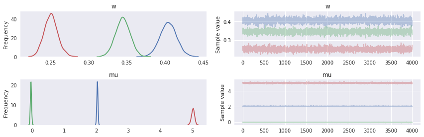
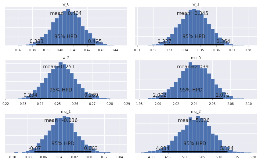
We see in the following plot that the posterior distribution on the weights and the component means has captured the true value quite well.

pm.traceplot(trace, varnames=['w', 'mu']);

/opt/conda/lib/python3.5/site-packages/matplotlib/font_manager.py:1297: UserWarning: findfont: Font family ['sans-serif'] not found. Falling back to DejaVu Sans
  (prop.get_family(), self.defaultFamily[fontext]))

pm.plot_posterior(trace, varnames=['w', 'mu']);

/opt/conda/lib/python3.5/site-packages/matplotlib/font_manager.py:1297: UserWarning: findfont: Font family ['sans-serif'] not found. Falling back to DejaVu Sans
  (prop.get_family(), self.defaultFamily[fontext]))

We can also sample from the model’s posterior predictive distribution, as follows.

with model:
    ppc_trace = pm.sample_ppc(trace, 5000, random_seed=SEED)

100%|██████████| 5000/5000 [03:28<00:00, 23.93it/s]

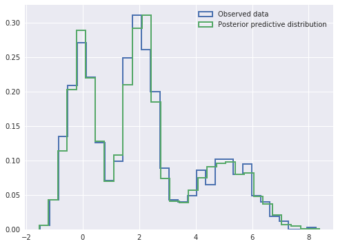
We see that the posterior predictive samples have a distribution quite close to that of the observed data.

fig, ax = plt.subplots(figsize=(8, 6))

ax.hist(x, bins=30, normed=True,
        histtype='step', lw=2,
        label='Observed data');
ax.hist(ppc_trace['x_obs'], bins=30, normed=True,
        histtype='step', lw=2,
        label='Posterior predictive distribution');

ax.legend(loc=1);

/opt/conda/lib/python3.5/site-packages/matplotlib/font_manager.py:1297: UserWarning: findfont: Font family ['sans-serif'] not found. Falling back to DejaVu Sans
  (prop.get_family(), self.defaultFamily[fontext]))