A Primer on Bayesian Methods for Multilevel Modeling
Hierarchical or multilevel modeling is a generalization of regression modeling.
Multilevel models are regression models in which the constituent model parameters are given probability models. This implies that model parameters are allowed to vary by group.
Observational units are often naturally clustered. Clustering induces dependence between observations, despite random sampling of clusters and random sampling within clusters.
A hierarchical model is a particular multilevel model where parameters are nested within one another.
Some multilevel structures are not hierarchical.
- e.g. “country” and “year” are not nested, but may represent separate, but overlapping, clusters of parameters
We will motivate this topic using an environmental epidemiology example.
Example: Radon contamination (Gelman and Hill 2006)
Radon is a radioactive gas that enters homes through contact points with the ground. It is a carcinogen that is the primary cause of lung cancer in non-smokers. Radon levels vary greatly from household to household.

radon
The EPA did a study of radon levels in 80,000 houses. Two important predictors:
- measurement in basement or first floor (radon higher in basements)
- county uranium level (positive correlation with radon levels)
We will focus on modeling radon levels in Minnesota.
The hierarchy in this example is households within county.
Data organization
First, we import the data from a local file, and extract Minnesota’s data.
In [1]:
%matplotlib inline
import numpy as np
import pandas as pd
import matplotlib.pyplot as plt
import seaborn as sns
sns.set_context('notebook')
sns.set_style('white')

from pymc3 import get_data

# Import radon data
srrs2 = pd.read_csv(get_data('srrs2.dat'))
srrs2.columns = srrs2.columns.map(str.strip)
srrs_mn = srrs2[srrs2.state=='MN'].copy()
Next, obtain the county-level predictor, uranium, by combining two variables.
In [2]:
srrs_mn['fips'] = srrs_mn.stfips*1000 + srrs_mn.cntyfips
cty = pd.read_csv(get_data('cty.dat'))
cty_mn = cty[cty.st=='MN'].copy()
cty_mn[ 'fips'] = 1000*cty_mn.stfips + cty_mn.ctfips
Use the merge method to combine home- and county-level information
in a single DataFrame.
In [3]:
srrs_mn = srrs_mn.merge(cty_mn[['fips', 'Uppm']], on='fips')
srrs_mn = srrs_mn.drop_duplicates(subset='idnum')
u = np.log(srrs_mn.Uppm)

n = len(srrs_mn)
In [4]:
srrs_mn.head()
Out[4]:
| idnum | state | state2 | stfips | zip | region | typebldg | floor | room | basement | ... | stopdt | activity | pcterr | adjwt | dupflag | zipflag | cntyfips | county | fips | Uppm | |
|---|---|---|---|---|---|---|---|---|---|---|---|---|---|---|---|---|---|---|---|---|---|
| 0 | 5081 | MN | MN | 27 | 55735 | 5 | 1 | 1 | 3 | N | ... | 12288 | 2.2 | 9.7 | 1146.499190 | 1 | 0 | 1 | AITKIN | 27001 | 0.502054 |
| 1 | 5082 | MN | MN | 27 | 55748 | 5 | 1 | 0 | 4 | Y | ... | 12088 | 2.2 | 14.5 | 471.366223 | 0 | 0 | 1 | AITKIN | 27001 | 0.502054 |
| 2 | 5083 | MN | MN | 27 | 55748 | 5 | 1 | 0 | 4 | Y | ... | 21188 | 2.9 | 9.6 | 433.316718 | 0 | 0 | 1 | AITKIN | 27001 | 0.502054 |
| 3 | 5084 | MN | MN | 27 | 56469 | 5 | 1 | 0 | 4 | Y | ... | 123187 | 1.0 | 24.3 | 461.623670 | 0 | 0 | 1 | AITKIN | 27001 | 0.502054 |
| 4 | 5085 | MN | MN | 27 | 55011 | 3 | 1 | 0 | 4 | Y | ... | 13088 | 3.1 | 13.8 | 433.316718 | 0 | 0 | 3 | ANOKA | 27003 | 0.428565 |
5 rows × 27 columns
We also need a lookup table (dict) for each unique county, for
indexing.
In [5]:
srrs_mn.county = srrs_mn.county.map(str.strip)
mn_counties = srrs_mn.county.unique()
counties = len(mn_counties)
county_lookup = dict(zip(mn_counties, range(len(mn_counties))))
Finally, create local copies of variables.
In [6]:
county = srrs_mn['county_code'] = srrs_mn.county.replace(county_lookup).values
radon = srrs_mn.activity
srrs_mn['log_radon'] = log_radon = np.log(radon + 0.1).values
floor_measure = srrs_mn.floor.values
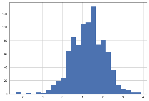
Distribution of radon levels in MN (log scale):
In [7]:
srrs_mn.activity.apply(lambda x: np.log(x+0.1)).hist(bins=25);
Conventional approaches
The two conventional alternatives to modeling radon exposure represent the two extremes of the bias-variance tradeoff:
*Complete pooling*:
Treat all counties the same, and estimate a single radon level.
*No pooling*:
Model radon in each county independently.
where \(j = 1,\ldots,85\)
The errors \(\epsilon_i\) may represent measurement error, temporal within-house variation, or variation among houses.
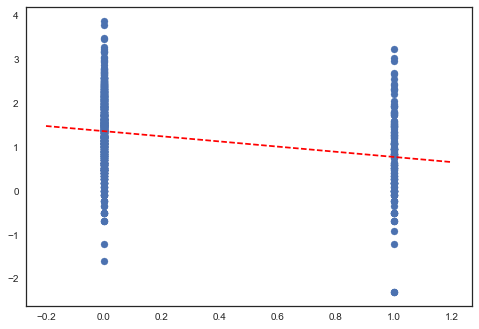
Here are the point estimates of the slope and intercept for the complete pooling model:
In [8]:
from pymc3 import Model, sample, Normal, HalfCauchy, Uniform

floor = srrs_mn.floor.values
log_radon = srrs_mn.log_radon.values

with Model() as pooled_model:

    beta = Normal('beta', 0, sd=1e5, shape=2)
    sigma = HalfCauchy('sigma', 5)

    theta = beta[0] + beta[1]*floor

    y = Normal('y', theta, sd=sigma, observed=log_radon)
In [9]:
with pooled_model:
    pooled_trace = sample(2000, n_init=50000, tune=1000)
Auto-assigning NUTS sampler...
Initializing NUTS using ADVI...
Average Loss = 1,121.1:  53%|█████▎    | 26617/50000 [00:03<00:03, 7258.34it/s]
Convergence archived at 27000
Interrupted at 27,000 [54%]: Average Loss = 1,201.3
100%|██████████| 2000/2000 [00:02<00:00, 798.65it/s]
In [10]:
b0, m0 = pooled_trace['beta', 1000:].mean(axis=0)
In [11]:
plt.scatter(srrs_mn.floor, np.log(srrs_mn.activity+0.1))
xvals = np.linspace(-0.2, 1.2)
plt.plot(xvals, m0*xvals+b0, 'r--');
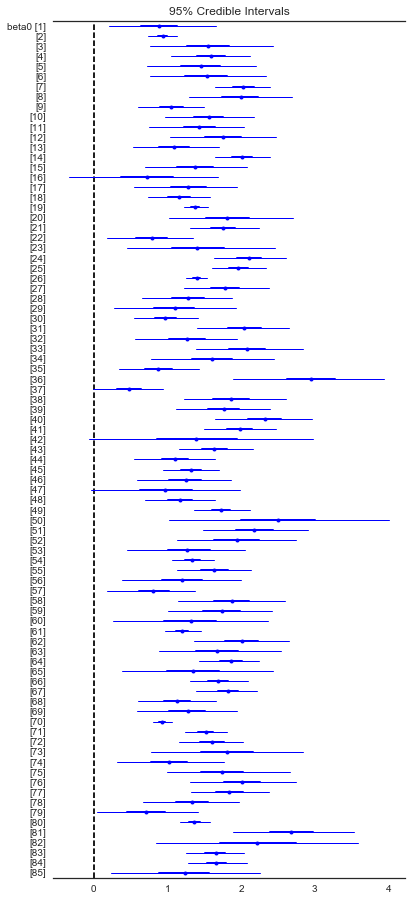
Estimates of county radon levels for the unpooled model:
In [12]:
with Model() as unpooled_model:

    beta0 = Normal('beta0', 0, sd=1e5, shape=counties)
    beta1 = Normal('beta1', 0, sd=1e5)
    sigma = HalfCauchy('sigma', 5)

    theta = beta0[county] + beta1*floor

    y = Normal('y', theta, sd=sigma, observed=log_radon)
In [14]:
with unpooled_model:
    unpooled_trace = sample(2000, n_init=50000, tune=1000)
Auto-assigning NUTS sampler...
Initializing NUTS using ADVI...
Average Loss = 2,069.3: 100%|██████████| 50000/50000 [00:11<00:00, 4504.30it/s]
Finished [100%]: Average Loss = 2,069.3
100%|██████████| 2000/2000 [00:13<00:00, 145.16it/s]
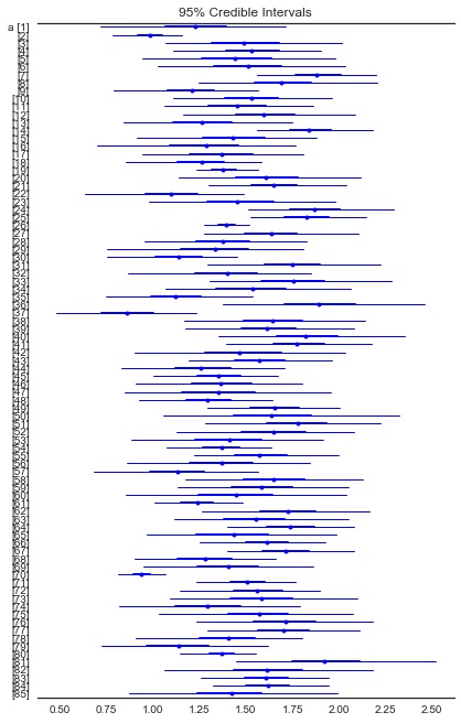
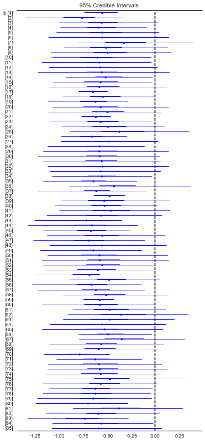
Here are the unpooled county expected values
In [15]:
from pymc3 import forestplot

plt.figure(figsize=(6,14))
forestplot(unpooled_trace, varnames=['beta0']);
In [16]:
unpooled_estimates = pd.Series(unpooled_trace['beta0'].mean(axis=0), index=mn_counties)
unpooled_se = pd.Series(unpooled_trace['beta0'].std(axis=0), index=mn_counties)
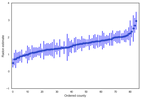
We can plot the ordered estimates to identify counties with high radon levels:
In [17]:
order = unpooled_estimates.order().index

plt.scatter(range(len(unpooled_estimates)), unpooled_estimates[order])
for i, m, se in zip(range(len(unpooled_estimates)), unpooled_estimates[order], unpooled_se[order]):
    plt.plot([i,i], [m-se, m+se], 'b-')
plt.xlim(-1,86); plt.ylim(-1,4)
plt.ylabel('Radon estimate');plt.xlabel('Ordered county');
/Users/fonnescj/anaconda3/envs/dev/lib/python3.6/site-packages/ipykernel_launcher.py:1: FutureWarning: order is deprecated, use sort_values(...)
  """Entry point for launching an IPython kernel.
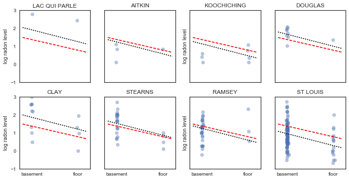
Here are visual comparisons between the pooled and unpooled estimates for a subset of counties representing a range of sample sizes.
In [18]:
sample_counties = ('LAC QUI PARLE', 'AITKIN', 'KOOCHICHING',
                    'DOUGLAS', 'CLAY', 'STEARNS', 'RAMSEY', 'ST LOUIS')

fig, axes = plt.subplots(2, 4, figsize=(12, 6), sharey=True, sharex=True)
axes = axes.ravel()
m = unpooled_trace['beta1'].mean()
for i,c in enumerate(sample_counties):
    y = srrs_mn.log_radon[srrs_mn.county==c]
    x = srrs_mn.floor[srrs_mn.county==c]
    axes[i].scatter(x + np.random.randn(len(x))*0.01, y, alpha=0.4)

    # No pooling model
    b = unpooled_estimates[c]

    # Plot both models and data
    xvals = np.linspace(-0.2, 1.2)
    axes[i].plot(xvals, m*xvals+b)
    axes[i].plot(xvals, m0*xvals+b0, 'r--')
    axes[i].set_xticks([0,1])
    axes[i].set_xticklabels(['basement', 'floor'])
    axes[i].set_ylim(-1, 3)
    axes[i].set_title(c)
    if not i%2:
        axes[i].set_ylabel('log radon level')
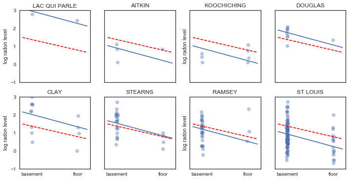
Neither of these models are satisfactory:
- if we are trying to identify high-radon counties, pooling is useless
- we do not trust extreme unpooled estimates produced by models using few observations
Multilevel and hierarchical models
When we pool our data, we imply that they are sampled from the same model. This ignores any variation among sampling units (other than sampling variance):

pooled
When we analyze data unpooled, we imply that they are sampled independently from separate models. At the opposite extreme from the pooled case, this approach claims that differences between sampling units are to large to combine them:

unpooled
In a hierarchical model, parameters are viewed as a sample from a population distribution of parameters. Thus, we view them as being neither entirely different or exactly the same. This is *parital pooling*.

hierarchical
We can use PyMC to easily specify multilevel models, and fit them using Markov chain Monte Carlo.
Partial pooling model
The simplest partial pooling model for the household radon dataset is one which simply estimates radon levels, without any predictors at any level. A partial pooling model represents a compromise between the pooled and unpooled extremes, approximately a weighted average (based on sample size) of the unpooled county estimates and the pooled estimates.
Estimates for counties with smaller sample sizes will shrink towards the state-wide average.
Estimates for counties with larger sample sizes will be closer to the unpooled county estimates.
In [19]:
with Model() as partial_pooling:

    # Priors
    mu_a = Normal('mu_a', mu=0., sd=1e5)
    sigma_a = HalfCauchy('sigma_a', 5)

    # Random intercepts
    a = Normal('a', mu=mu_a, sd=sigma_a, shape=counties)

    # Model error
    sigma_y = HalfCauchy('sigma_y',5)

    # Expected value
    y_hat = a[county]

    # Data likelihood
    y_like = Normal('y_like', mu=y_hat, sd=sigma_y, observed=log_radon)
In [20]:
with partial_pooling:
    partial_pooling_trace = sample(2000, n_init=50000, tune=1000)
Auto-assigning NUTS sampler...
Initializing NUTS using ADVI...
Average Loss = 1,115.5: 100%|██████████| 50000/50000 [00:13<00:00, 3590.55it/s]
Finished [100%]: Average Loss = 1,115.5
100%|██████████| 2000/2000 [00:07<00:00, 253.79it/s]
In [21]:
sample_trace = partial_pooling_trace['a', 1000:]

fig, axes = plt.subplots(1, 2, figsize=(14,6), sharex=True, sharey=True)
samples, counties = sample_trace.shape
jitter = np.random.normal(scale=0.1, size=counties)

n_county = srrs_mn.groupby('county')['idnum'].count()
unpooled_means = srrs_mn.groupby('county')['log_radon'].mean()
unpooled_sd = srrs_mn.groupby('county')['log_radon'].std()
unpooled = pd.DataFrame({'n':n_county, 'm':unpooled_means, 'sd':unpooled_sd})
unpooled['se'] = unpooled.sd/np.sqrt(unpooled.n)

axes[0].plot(unpooled.n + jitter, unpooled.m, 'b.')
for j, row in zip(jitter, unpooled.iterrows()):
    name, dat = row
    axes[0].plot([dat.n+j,dat.n+j], [dat.m-dat.se, dat.m+dat.se], 'b-')
axes[0].set_xscale('log')
axes[0].hlines(sample_trace.mean(), 0.9, 100, linestyles='--')


samples, counties = sample_trace.shape
means = sample_trace.mean(axis=0)
sd = sample_trace.std(axis=0)
axes[1].scatter(n_county.values + jitter, means)
axes[1].set_xscale('log')
axes[1].set_xlim(1,100)
axes[1].set_ylim(0, 3)
axes[1].hlines(sample_trace.mean(), 0.9, 100, linestyles='--')
for j,n,m,s in zip(jitter, n_county.values, means, sd):
    axes[1].plot([n+j]*2, [m-s, m+s], 'b-')
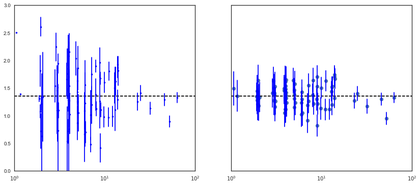
Notice the difference between the unpooled and partially-pooled estimates, particularly at smaller sample sizes. The former are both more extreme and more imprecise.
Varying intercept model
This model allows intercepts to vary across county, according to a random effect.
where
and the intercept random effect:
As with the the “no-pooling” model, we set a separate intercept for each county, but rather than fitting separate least squares regression models for each county, multilevel modeling shares strength among counties, allowing for more reasonable inference in counties with little data.
In [22]:
with Model() as varying_intercept:

    # Priors
    mu_a = Normal('mu_a', mu=0., tau=0.0001)
    sigma_a = HalfCauchy('sigma_a', 5)


    # Random intercepts
    a = Normal('a', mu=mu_a, sd=sigma_a, shape=counties)
    # Common slope
    b = Normal('b', mu=0., sd=1e5)

    # Model error
    sd_y = HalfCauchy('sd_y', 5)

    # Expected value
    y_hat = a[county] + b * floor_measure

    # Data likelihood
    y_like = Normal('y_like', mu=y_hat, sd=sd_y, observed=log_radon)
We can fit the above model using MCMC.
In [23]:
with varying_intercept:
    varying_intercept_trace = sample(2000, n_init=50000, tune=1000)
Auto-assigning NUTS sampler...
Initializing NUTS using ADVI...
Average Loss = 1,077.4: 100%|██████████| 50000/50000 [00:11<00:00, 4206.38it/s]
Finished [100%]: Average Loss = 1,077.5
100%|██████████| 2000/2000 [00:06<00:00, 296.67it/s]
In [24]:
from pymc3 import forestplot, traceplot, plot_posterior

plt.figure(figsize=(6,14))
forestplot(varying_intercept_trace[1000:], varnames=['a'])
Out[24]:
<matplotlib.gridspec.GridSpec at 0x12feda6d8>
In [25]:
plot_posterior(varying_intercept_trace[1000:], varnames=['sigma_a', 'b'])
Out[25]:
array([<matplotlib.axes._subplots.AxesSubplot object at 0x1307c6d68>,
       <matplotlib.axes._subplots.AxesSubplot object at 0x1308f4710>], dtype=object)
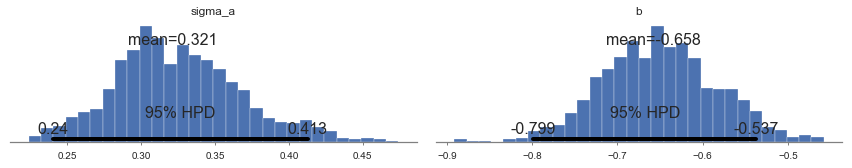
The estimate for the floor coefficient is approximately -0.66, which
can be interpreted as houses without basements having about half
(\(\exp(-0.66) = 0.52\)) the radon levels of those with basements,
after accounting for county.
In [26]:
from pymc3 import summary

summary(varying_intercept_trace, varnames=['b'])
b:

  Mean             SD               MC Error         95% HPD interval
  -------------------------------------------------------------------

  -0.660           0.068            0.002            [-0.794, -0.532]

  Posterior quantiles:
  2.5            25             50             75             97.5
  |--------------|==============|==============|--------------|

  -0.787         -0.706         -0.661         -0.615         -0.525
In [27]:
xvals = np.arange(2)
bp = varying_intercept_trace[a, 1000:].mean(axis=0)
mp = varying_intercept_trace[b, 1000:].mean()
for bi in bp:
    plt.plot(xvals, mp*xvals + bi, 'bo-', alpha=0.4)
plt.xlim(-0.1,1.1);
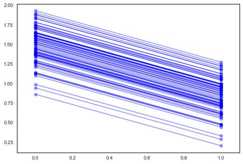
It is easy to show that the partial pooling model provides more objectively reasonable estimates than either the pooled or unpooled models, at least for counties with small sample sizes.
In [28]:
fig, axes = plt.subplots(2, 4, figsize=(12, 6), sharey=True, sharex=True)
axes = axes.ravel()
for i,c in enumerate(sample_counties):

    # Plot county data
    y = srrs_mn.log_radon[srrs_mn.county==c]
    x = srrs_mn.floor[srrs_mn.county==c]
    axes[i].scatter(x + np.random.randn(len(x))*0.01, y, alpha=0.4)

    # No pooling model
    m,b = unpooled_estimates[['floor', c]]

    xvals = np.linspace(-0.2, 1.2)
    # Unpooled estimate
    axes[i].plot(xvals, m*xvals+b)
    # Pooled estimate
    axes[i].plot(xvals, m0*xvals+b0, 'r--')
    # Partial pooling esimate
    axes[i].plot(xvals, mp*xvals+bp[county_lookup[c]], 'k:')
    axes[i].set_xticks([0,1])
    axes[i].set_xticklabels(['basement', 'floor'])
    axes[i].set_ylim(-1, 3)
    axes[i].set_title(c)
    if not i%2:
        axes[i].set_ylabel('log radon level')
Varying slope model
Alternatively, we can posit a model that allows the counties to vary according to how the location of measurement (basement or floor) influences the radon reading.
In [29]:
with Model() as varying_slope:

    # Priors
    mu_b = Normal('mu_b', mu=0., sd=1e5)
    sigma_b = HalfCauchy('sigma_b', 5)

    # Common intercepts
    a = Normal('a', mu=0., sd=1e5)
    # Random slopes
    b = Normal('b', mu=mu_b, sd=sigma_b, shape=counties)

    # Model error
    sigma_y = HalfCauchy('sigma_y',5)

    # Expected value
    y_hat = a + b[county] * floor_measure

    # Data likelihood
    y_like = Normal('y_like', mu=y_hat, sd=sigma_y, observed=log_radon)
In [30]:
with varying_slope:
    varying_slope_trace = sample(2000, n_init=50000, tune=1000)
Auto-assigning NUTS sampler...
Initializing NUTS using ADVI...
Average Loss = 1,124.6: 100%|██████████| 50000/50000 [00:13<00:00, 3759.25it/s]
Finished [100%]: Average Loss = 1,124.6
100%|█████████▉| 1998/2000 [00:12<00:00, 172.69it/s]/Users/fonnescj/Repos/pymc3/pymc3/step_methods/hmc/nuts.py:268: UserWarning: The acceptance probability in chain 0 does not match the target. It is 0.655412161099, but should be close to 0.8. Try to increase the number of tuning steps.
  % (chain, mean_accept, target_accept))
100%|██████████| 2000/2000 [00:12<00:00, 160.72it/s]
In [38]:
plt.figure(figsize=(6,14))
forestplot(varying_slope_trace[1000:], varnames=['b'])
Out[38]:
<matplotlib.gridspec.GridSpec at 0x13497aef0>
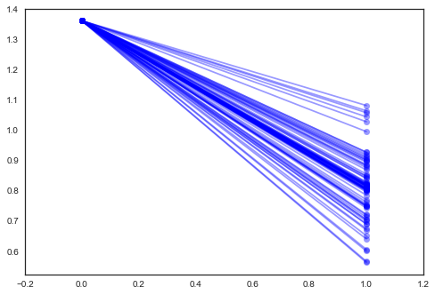
In [32]:
xvals = np.arange(2)
b = varying_slope_trace['a', 1000:].mean()
m = varying_slope_trace['b', 1000:].mean(axis=0)
for mi in m:
    plt.plot(xvals, mi*xvals + b, 'bo-', alpha=0.4)
plt.xlim(-0.2, 1.2);
Varying intercept and slope model
The most general model allows both the intercept and slope to vary by county:
In [33]:
with Model() as varying_intercept_slope:

    # Priors
    mu_a = Normal('mu_a', mu=0., sd=1e5)
    sigma_a = HalfCauchy('sigma_a', 5)
    mu_b = Normal('mu_b', mu=0., sd=1e5)
    sigma_b = HalfCauchy('sigma_b', 5)

    # Random intercepts
    a = Normal('a', mu=mu_a, sd=sigma_a, shape=counties)
    # Random slopes
    b = Normal('b', mu=mu_b, sd=sigma_b, shape=counties)

    # Model error
    sigma_y = Uniform('sigma_y', lower=0, upper=100)

    # Expected value
    y_hat = a[county] + b[county] * floor_measure

    # Data likelihood
    y_like = Normal('y_like', mu=y_hat, sd=sigma_y, observed=log_radon)
In [34]:
with varying_intercept_slope:
    varying_intercept_slope_trace = sample(2000, n_init=50000, tune=1000)
Auto-assigning NUTS sampler...
Initializing NUTS using ADVI...
Average Loss = 1,093.1: 100%|██████████| 50000/50000 [00:19<00:00, 2551.95it/s]
Finished [100%]: Average Loss = 1,093.1
100%|██████████| 2000/2000 [00:17<00:00, 116.26it/s]
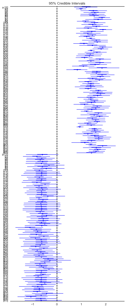
In [35]:
plt.figure(figsize=(6,16))
forestplot(varying_intercept_slope_trace[1000:], varnames=['a','b'])
Out[35]:
<matplotlib.gridspec.GridSpec at 0x12fd556d8>
In [36]:
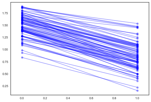
xvals = np.arange(2)
b = varying_intercept_slope_trace['a', 1000:].mean(axis=0)
m = varying_intercept_slope_trace['b', 1000:].mean(axis=0)
for bi,mi in zip(b,m):
    plt.plot(xvals, mi*xvals + bi, 'bo-', alpha=0.4)
plt.xlim(-0.1, 1.1);
Adding group-level predictors
A primary strength of multilevel models is the ability to handle predictors on multiple levels simultaneously. If we consider the varying-intercepts model above:
we may, instead of a simple random effect to describe variation in the expected radon value, specify another regression model with a county-level covariate. Here, we use the county uranium reading \(u_j\), which is thought to be related to radon levels:
Thus, we are now incorporating a house-level predictor (floor or basement) as well as a county-level predictor (uranium).
Note that the model has both indicator variables for each county, plus a county-level covariate. In classical regression, this would result in collinearity. In a multilevel model, the partial pooling of the intercepts towards the expected value of the group-level linear model avoids this.
Group-level predictors also serve to reduce group-level variation \(\sigma_{\alpha}\). An important implication of this is that the group-level estimate induces stronger pooling.
In [39]:
from pymc3 import Deterministic

with Model() as hierarchical_intercept:

    # Priors
    sigma_a = HalfCauchy('sigma_a', 5)

    # County uranium model for slope
    gamma_0 = Normal('gamma_0', mu=0., sd=1e5)
    gamma_1 = Normal('gamma_1', mu=0., sd=1e5)


    # Uranium model for intercept
    mu_a = gamma_0 + gamma_1*u
    # County variation not explained by uranium
    eps_a = Normal('eps_a', mu=0, sd=sigma_a, shape=counties)
    a = Deterministic('a', mu_a + eps_a[county])

    # Common slope
    b = Normal('b', mu=0., sd=1e5)

    # Model error
    sigma_y = Uniform('sigma_y', lower=0, upper=100)

    # Expected value
    y_hat = a + b * floor_measure

    # Data likelihood
    y_like = Normal('y_like', mu=y_hat, sd=sigma_y, observed=log_radon)
In [40]:
with hierarchical_intercept:
    hierarchical_intercept_trace = sample(2000, n_init=50000, tune=1000)
Auto-assigning NUTS sampler...
Initializing NUTS using ADVI...
Average Loss = 1,081.6: 100%|██████████| 50000/50000 [00:12<00:00, 3866.91it/s]
Finished [100%]: Average Loss = 1,081.6
100%|██████████| 2000/2000 [00:08<00:00, 228.08it/s]
In [41]:
a_means = hierarchical_intercept_trace['a', 1000:].mean(axis=0)
plt.scatter(u, a_means)
g0 = hierarchical_intercept_trace['gamma_0'].mean()
g1 = hierarchical_intercept_trace['gamma_1'].mean()
xvals = np.linspace(-1, 0.8)
plt.plot(xvals, g0+g1*xvals, 'k--')
plt.xlim(-1, 0.8)

a_se = hierarchical_intercept_trace['a', 1000:].std(axis=0)
for ui, m, se in zip(u, a_means, a_se):
    plt.plot([ui,ui], [m-se, m+se], 'b-')
plt.xlabel('County-level uranium'); plt.ylabel('Intercept estimate');
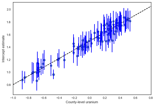
The standard errors on the intercepts are narrower than for the partial-pooling model without a county-level covariate.
Correlations among levels
In some instances, having predictors at multiple levels can reveal correlation between individual-level variables and group residuals. We can account for this by including the average of the individual predictors as a covariate in the model for the group intercept.
These are broadly referred to as *contextual effects*.
In [42]:
# Create new variable for mean of floor across counties
xbar = srrs_mn.groupby('county')['floor'].mean().rename(county_lookup).values
In [43]:
with Model() as contextual_effect:

    # Priors
    sigma_a = HalfCauchy('sigma_a', 5)

    # County uranium model for slope
    gamma = Normal('gamma', mu=0., sd=1e5, shape=3)

    # Uranium model for intercept
    mu_a = Deterministic('mu_a', gamma[0] + gamma[1]*u.values + gamma[2]*xbar[county])

    # County variation not explained by uranium
    eps_a = Normal('eps_a', mu=0, sd=sigma_a, shape=counties)
    a = Deterministic('a', mu_a + eps_a[county])

    # Common slope
    b = Normal('b', mu=0., sd=1e15)

    # Model error
    sigma_y = Uniform('sigma_y', lower=0, upper=100)

    # Expected value
    y_hat = a + b * floor_measure

    # Data likelihood
    y_like = Normal('y_like', mu=y_hat, sd=sigma_y, observed=log_radon)
In [44]:
with contextual_effect:
    contextual_effect_trace = sample(2000, n_init=50000, tune=1000)
Auto-assigning NUTS sampler...
Initializing NUTS using ADVI...
Average Loss = 1,116.3: 100%|██████████| 50000/50000 [00:12<00:00, 4108.64it/s]
Finished [100%]: Average Loss = 1,116.3
100%|██████████| 2000/2000 [00:11<00:00, 168.51it/s]
In [45]:
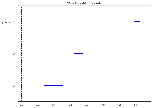
forestplot(contextual_effect_trace[1000:], varnames=['gamma'])
Out[45]:
<matplotlib.gridspec.GridSpec at 0x132e21b00>
In [46]:
summary(contextual_effect_trace[1000:], varnames=['gamma'])
gamma:

  Mean             SD               MC Error         95% HPD interval
  -------------------------------------------------------------------

  1.424            0.047            0.003            [1.337, 1.519]
  0.697            0.081            0.003            [0.537, 0.853]
  0.395            0.183            0.010            [0.026, 0.754]

  Posterior quantiles:
  2.5            25             50             75             97.5
  |--------------|==============|==============|--------------|

  1.335          1.392          1.424          1.456          1.519
  0.537          0.645          0.696          0.752          0.853
  0.015          0.281          0.396          0.513          0.753
So, we might infer from this that counties with higher proportions of houses without basements tend to have higher baseline levels of radon. Perhaps this is related to the soil type, which in turn might influence what type of structures are built.
Prediction
Gelman (2006) used cross-validation tests to check the prediction error of the unpooled, pooled, and partially-pooled models
root mean squared cross-validation prediction errors:
- unpooled = 0.86
- pooled = 0.84
- multilevel = 0.79
There are two types of prediction that can be made in a multilevel model:
- a new individual within an existing group
- a new individual within a new group
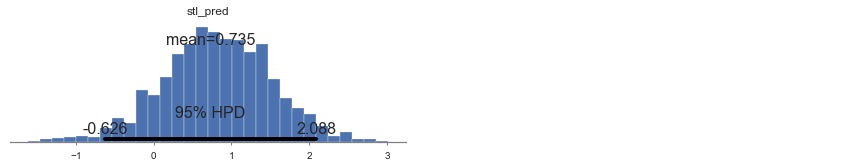
For example, if we wanted to make a prediction for a new house with no basement in St. Louis county, we just need to sample from the radon model with the appropriate intercept.
In [47]:
county_lookup['ST LOUIS']
Out[47]:
69
That is,
This is simply a matter of adding a single additional line in PyMC:
In [48]:
with Model() as contextual_pred:

    # Priors
    sigma_a = HalfCauchy('sigma_a', 5)

    # County uranium model for slope
    gamma = Normal('gamma', mu=0., sd=1e5, shape=3)

    # Uranium model for intercept
    mu_a = Deterministic('mu_a', gamma[0] + gamma[1]*u.values + gamma[2]*xbar[county])

    # County variation not explained by uranium
    eps_a = Normal('eps_a', mu=0, sd=sigma_a, shape=counties)
    a = Deterministic('a', mu_a + eps_a[county])

    # Common slope
    b = Normal('b', mu=0., sd=1e15)

    # Model error
    sigma_y = Uniform('sigma_y', lower=0, upper=100)

    # Expected value
    y_hat = a + b * floor_measure

    # Data likelihood
    y_like = Normal('y_like', mu=y_hat, sd=sigma_y, observed=log_radon)

    # St Louis county prediction
    stl_pred = Normal('stl_pred', mu=a[69] + b, sd=sigma_y)
In [49]:
with contextual_pred:
    contextual_pred_trace = sample(2000, n_init=50000, tune=1000)
Auto-assigning NUTS sampler...
Initializing NUTS using ADVI...
Average Loss = 1,116.3: 100%|██████████| 50000/50000 [00:12<00:00, 3890.22it/s]
Finished [100%]: Average Loss = 1,116.3
100%|██████████| 2000/2000 [00:15<00:00, 131.23it/s]
In [50]:
plot_posterior(contextual_pred_trace[1000:], varnames=['stl_pred'])
Out[50]:
array([<matplotlib.axes._subplots.AxesSubplot object at 0x12d950208>], dtype=object)
Benefits of Multilevel Models
Accounting for natural hierarchical structure of observational data
Estimation of coefficients for (under-represented) groups
Incorporating individual- and group-level information when estimating group-level coefficients
Allowing for variation among individual-level coefficients across groups
References
Gelman, A., & Hill, J. (2006). Data Analysis Using Regression and Multilevel/Hierarchical Models (1st ed.). Cambridge University Press.
Gelman, A. (2006). Multilevel (Hierarchical) modeling: what it can and cannot do. Technometrics, 48(3), 432–435.