Stochastic Volatility model
In [1]:
import numpy as np
import pymc3 as pm
from pymc3.distributions.timeseries import GaussianRandomWalk

from scipy import optimize

%pylab inline
Populating the interactive namespace from numpy and matplotlib
Asset prices have time-varying volatility (variance of day over day
returns). In some periods, returns are highly variable, while in
others very stable. Stochastic volatility models model this with a
latent volatility variable, modeled as a stochastic process. The
following model is similar to the one described in the No-U-Turn Sampler
paper, Hoffman (2011) p21.
Here, \(y\) is the daily return series and \(s\) is the latent log volatility process.
Build Model
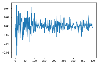
First we load some daily returns of the S&P 500.
In [2]:
n = 400
returns = np.genfromtxt(pm.get_data("SP500.csv"))[-n:]
returns[:5]
Out[2]:
array([-0.00637 , -0.004045, -0.02547 , 0.005102, -0.047733])
In [3]:
plt.plot(returns)
Out[3]:
[<matplotlib.lines.Line2D at 0x7fae8c869a20>]
Specifying the model in pymc3 mirrors its statistical specification.
In [4]:
model = pm.Model()
with model:
    sigma = pm.Exponential('sigma', 1./.02, testval=.1)

    nu = pm.Exponential('nu', 1./10)
    s = GaussianRandomWalk('s', sigma**-2, shape=n)

    r = pm.StudentT('r', nu, lam=pm.math.exp(-2*s), observed=returns)
Fit Model
For this model, the full maximum a posteriori (MAP) point is degenerate and has infinite density. To get good convergence with NUTS we use ADVI (autodiff variational inference) for initialization.
In [9]:
with model:
    trace = pm.sample(2000, tune=1000)[1000:]
Auto-assigning NUTS sampler...
Initializing NUTS using ADVI...
Average Loss = 7.9136: 100%|██████████| 200000/200000 [01:14<00:00, 2691.66it/s]
Finished [100%]: Average Loss = 7.896
100%|██████████| 2000/2000 [04:47<00:00,  8.48it/s]/home/jovyan/pymc3/pymc3/step_methods/hmc/nuts.py:255: UserWarning: Chain 0 reached the maximum tree depth. Increase max_treedepth, increase target_accept or reparameterize.
  'reparameterize.' % chain)
/home/jovyan/pymc3/pymc3/step_methods/hmc/nuts.py:268: UserWarning: The acceptance probability in chain 0 does not match the target. It is 0.688505126364, but should be close to 0.8. Try to increase the number of tuning steps.
  % (chain, mean_accept, target_accept))
In [10]:
figsize(12,6)
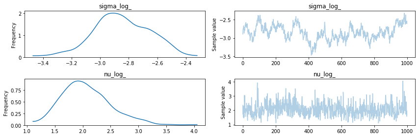
pm.traceplot(trace, model.vars[:-1]);
In [11]:
figsize(12,6)
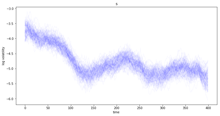
title(str(s))
plot(trace[s][::10].T, 'b', alpha=.03);
xlabel('time')
ylabel('log volatility')
Out[11]:
<matplotlib.text.Text at 0x7fae6019f8d0>
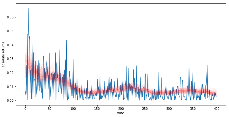
Looking at the returns over time and overlaying the estimated standard deviation we can see how the model tracks the volatility over time.
In [12]:
plot(np.abs(returns))
plot(np.exp(trace[s][::10].T), 'r', alpha=.03);
sd = np.exp(trace[s].T)
xlabel('time')
ylabel('absolute returns')
Out[12]:
<matplotlib.text.Text at 0x7fae64197c50>
References
- Hoffman & Gelman. (2011). The No-U-Turn Sampler: Adaptively Setting Path Lengths in Hamiltonian Monte Carlo.