Variational API quickstart
VI API is focused on solving regular problems when utilizing posterior distributions. Common usecases that can be solved with this module are the following:
- Get Random Generator that samples from posterior and computes some expression
- Get Monte Carlo approximation of expectation, variance and other statistics
- Remove symbolic dependence on PyMC3 random nodes and be able to call
.eval() - Make a bridge to arbitrary theano code
Sounds good, doesn’t it?
Moreover there are a lot of inference methods that have similar API so you are free to choose what fits the best for the problem
In [1]:
%matplotlib inline
import matplotlib.pyplot as plt
import pymc3 as pm
import theano
import numpy as np
np.random.seed(42)
pm.set_tt_rng(42)
Basic setup
We do not need complex models to play with VI API, instead we’ll have a simple mixture model
In [2]:
w = pm.floatX([.2, .8])
mu = pm.floatX([-.3, .5])
sd = pm.floatX([.1, .1])
with pm.Model() as model:
    x = pm.NormalMixture('x', w=w, mu=mu, sd=sd, dtype=theano.config.floatX)
    x2 = x ** 2
    sin_x = pm.math.sin(x)
We can’t compute analytical expectations quickly here. Instead we can get approximations for it with MC methods. Lets use NUTS first. It required these variables to be in deterministic list
In [3]:
with model:
    pm.Deterministic('x2', x2)
    pm.Deterministic('sin_x', sin_x)
In [4]:
with model:
    trace = pm.sample(50000)
Auto-assigning NUTS sampler...
Initializing NUTS using ADVI...
Average Loss = 5.7775:   1%|          | 1941/200000 [00:00<00:21, 9272.58it/s]
Convergence archived at 2900
Interrupted at 2,900 [1%]: Average Loss = 6.0938
100%|██████████| 50500/50500 [00:24<00:00, 2071.58it/s]
In [5]:
pm.traceplot(trace);
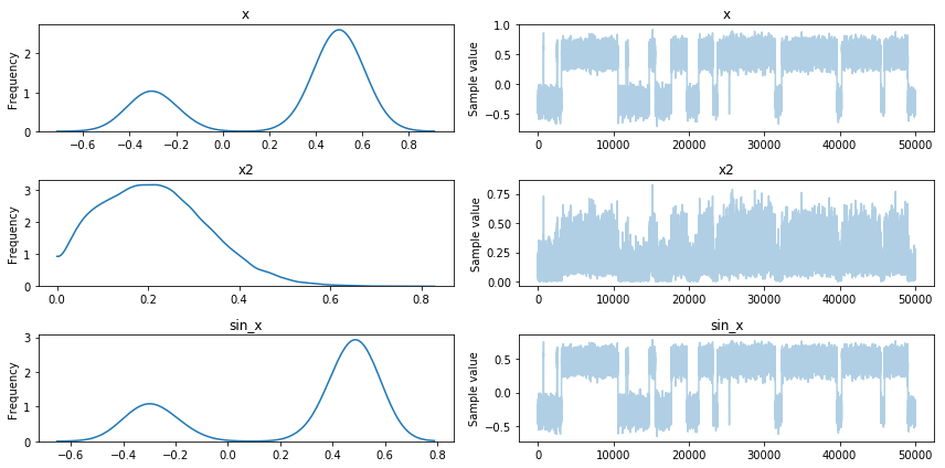
Looks good, we can see multimodality matters. Moreover we have samples
for \(x^2\) and \(sin(x)\). There is one drawback, you should
know in advance what exactly you want to see in trace and call
Deterministic(.) on it.
VI API is about the opposite approach. You do inference on model, then experiments come after. Let’s do the same setup without deterministics
In [6]:
with pm.Model() as model:
    x = pm.NormalMixture('x', w=w, mu=mu, sd=sd, dtype=theano.config.floatX)
    x2 = x ** 2
    sin_x = pm.math.sin(x)
And calculate ADVI approximation
In [7]:
with model:
    mean_field = pm.fit(method='advi')
Average Loss = 2.2413: 100%|██████████| 10000/10000 [00:00<00:00, 11143.17it/s]
Finished [100%]: Average Loss = 2.2687
In [8]:
pm.plot_posterior(mean_field.sample(1000));
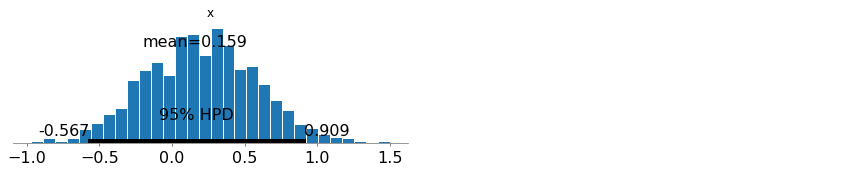
You can see no multimodality here. ADVI will fail to approximate multimodal distribution as it uses simple Gaussian distribution that has a single mode.
Notice that we did a lot more iterations as we did not check convergence of inference. That can be done via callbacks.
In [9]:
help(pm.callbacks.CheckParametersConvergence)
Help on class CheckParametersConvergence in module pymc3.variational.callbacks:

class CheckParametersConvergence(Callback)
 |  Convergence stopping check
 |
 |  Parameters
 |  ----------
 |  every : int
 |      check frequency
 |  tolerance : float
 |      if diff norm < tolerance : break
 |  diff : str
 |      difference type one of {'absolute', 'relative'}
 |  ord : {non-zero int, inf, -inf, 'fro', 'nuc'}, optional
 |      see more info in :func:`numpy.linalg.norm`
 |
 |  Examples
 |  --------
 |  >>> with model:
 |  ...     approx = pm.fit(
 |  ...         n=10000, callbacks=[
 |  ...             CheckParametersConvergence(
 |  ...                 every=50, diff='absolute',
 |  ...                 tolerance=1e-4)
 |  ...         ]
 |  ...     )
 |
 |  Method resolution order:
 |      CheckParametersConvergence
 |      Callback
 |      builtins.object
 |
 |  Methods defined here:
 |
 |  __call__(self, approx, _, i)
 |      Call self as a function.
 |
 |  __init__(self, every=100, tolerance=0.001, diff='relative', ord=inf)
 |      Initialize self.  See help(type(self)) for accurate signature.
 |
 |  ----------------------------------------------------------------------
 |  Static methods defined here:
 |
 |  flatten_shared(shared_list)
 |
 |  ----------------------------------------------------------------------
 |  Data descriptors inherited from Callback:
 |
 |  __dict__
 |      dictionary for instance variables (if defined)
 |
 |  __weakref__
 |      list of weak references to the object (if defined)
Let’s use defaults as they seem to be reasonable
In [10]:
with model:
    mean_field = pm.fit(method='advi', callbacks=[pm.callbacks.CheckParametersConvergence()])
Average Loss = 2.2559: 100%|██████████| 10000/10000 [00:01<00:00, 9938.76it/s]
Finished [100%]: Average Loss = 2.2763
In [11]:
plt.plot(mean_field.hist);
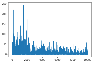
Hmm, something went wrong, we again did a lot of iterations. The reason is that mean of ADVI approximation is close to 0 and taking relative difference is unstable for checking convergence
In [12]:
with model:
    mean_field = pm.fit(method='advi', callbacks=[pm.callbacks.CheckParametersConvergence(diff='absolute')])
Average Loss = 3.6063:  40%|████      | 4029/10000 [00:00<00:00, 10150.26it/s]
Convergence archived at 4700
Interrupted at 4,700 [47%]: Average Loss = 4.7995
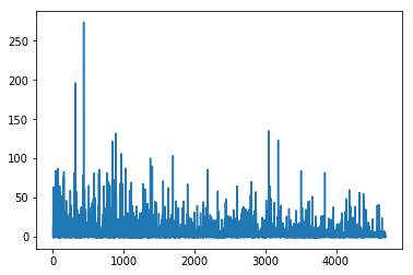
We can access inference history via .hist attribute.
In [13]:
plt.plot(mean_field.hist);
Tracking parameters
That’s much better. There is another usefull callback in pymc3. It
allows tracking of arbitrary statistics during inference. One of them
(but sometimes memory consuming) is tracking parameters. In function
pm.fit we do not have direct access to approximation before
inference. But tracking parameters requires it. To cope with this
problem we can use Object Oriented API for inference.
In [14]:
with model:
    advi = pm.ADVI()
In [15]:
advi.approx
Out[15]:
<pymc3.variational.approximations.MeanField at 0x11c9444e0>
Different approximations have different parameters. In MeanField case we use \(\rho\) and \(\mu\) (inspired by Bayes by BackProp)
In [16]:
advi.approx.shared_params
Out[16]:
{'mu': mu, 'rho': rho}
But having convinient shortcuts happens to be usefull sometimes. One of most frequent cases is specifying mass matrix for NUTS
In [17]:
advi.approx.mean.eval(), advi.approx.std.eval()
Out[17]:
(array([ 0.34], dtype=float32), array([ 0.69314718], dtype=float32))
That’s what we want
In [18]:
tracker = pm.callbacks.Tracker(
    mean=advi.approx.mean.eval,  # callable that returns mean
    std=advi.approx.std.eval  # callable that returns std
)
In [19]:
print(pm.callbacks.Tracker.__doc__)
    Helper class to record arbitrary stats during VI

    It is possible to pass a function that takes no arguments
    If call fails then (approx, hist, i) are passed


    Parameters
    ----------
    kwargs : key word arguments
        keys mapping statname to callable that records the stat

    Examples
    --------
    Consider we want time on each iteration
    >>> import time
    >>> tracker = Tracker(time=time.time)
    >>> with model:
    ...     approx = pm.fit(callbacks=[tracker])

    Time can be accessed via :code:`tracker['time']` now
    For more complex summary one can use callable that takes
    (approx, hist, i) as arguments
    >>> with model:
    ...     my_callable = lambda ap, h, i: h[-1]
    ...     tracker = Tracker(some_stat=my_callable)
    ...     approx = pm.fit(callbacks=[tracker])

    Multiple stats are valid too
    >>> with model:
    ...     tracker = Tracker(some_stat=my_callable, time=time.time)
    ...     approx = pm.fit(callbacks=[tracker])
Now, calling advi.fit will make inference but in a slightly more
flexible way.
In [20]:
approx = advi.fit(20000, callbacks=[tracker])
Average Loss = 1.9568: 100%|██████████| 20000/20000 [00:02<00:00, 7952.04it/s]
Finished [100%]: Average Loss = 1.9589
We can now plot inference results and trace for parameters
In [21]:
fig = plt.figure(figsize=(16, 9))
mu_ax = fig.add_subplot(221)
std_ax = fig.add_subplot(222)
hist_ax = fig.add_subplot(212)
mu_ax.plot(tracker['mean'])
mu_ax.set_title('Mean track')
std_ax.plot(tracker['std'])
std_ax.set_title('Std track')
hist_ax.plot(advi.hist)
hist_ax.set_title('Negative ELBO track');
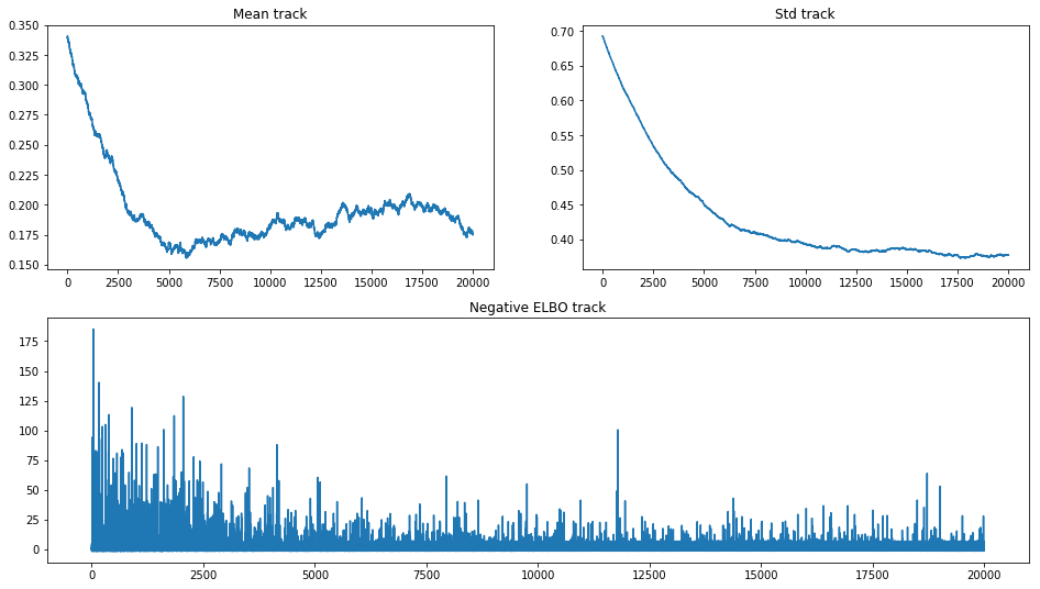
That picture is very informative. We can see how poor mean converges and that different values for it do not change elbo significantly. As we are using OO API, we can continue inference to get some visual convergence
In [22]:
approx = advi.fit(100000, callbacks=[tracker])
Average Loss = 1.8638: 100%|██████████| 100000/100000 [00:17<00:00, 5645.84it/s]
Finished [100%]: Average Loss = 1.8422
And this picture again
In [23]:
fig = plt.figure(figsize=(16, 9))
mu_ax = fig.add_subplot(221)
std_ax = fig.add_subplot(222)
hist_ax = fig.add_subplot(212)
mu_ax.plot(tracker['mean'])
mu_ax.set_title('Mean track')
std_ax.plot(tracker['std'])
std_ax.set_title('Std track')
hist_ax.plot(advi.hist)
hist_ax.set_title('Negative ELBO track');
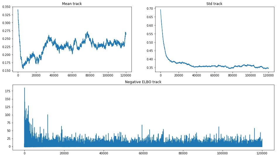
Eventually mean went up and started to behave like a random walk. We
are still uncertain for the true optimum of ADVI inference. Such picture
can be an evidence for poor algorithm chosen to make inference on the
model. It is unstable and can produce significantly different results
with different random seeds even.
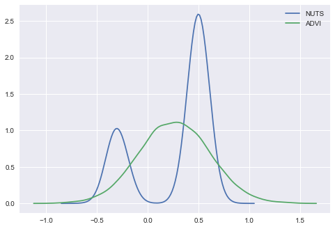
Let’s compare results with old NUTS trace
In [24]:
import seaborn as sns
ax = sns.kdeplot(trace['x'], label='NUTS');
sns.kdeplot(approx.sample(10000)['x'], label='ADVI');
To cope with multimodality we can instead use SVGD that creates approximation based on large number of particles
In [25]:
with model:
    svgd_approx = pm.fit(300, method='svgd', inf_kwargs=dict(n_particles=1000),
                         obj_optimizer=pm.sgd(learning_rate=0.01))
100%|██████████| 300/300 [00:39<00:00, 7.55it/s]
In [26]:
ax = sns.kdeplot(trace['x'], label='NUTS');
sns.kdeplot(approx.sample(10000)['x'], label='ADVI');
sns.kdeplot(svgd_approx.sample(2000)['x'], label='SVGD');
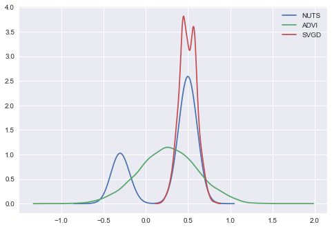
Seems like our SVGD got stuck in the mode. The reason is just bad
initialization. We can solve the problem using larger jitter in init
In [27]:
with model:
    svgd_approx = pm.fit(300, method='svgd',
                         inf_kwargs=dict(n_particles=1000, jitter=1),
                         obj_optimizer=pm.sgd(learning_rate=0.01))
100%|██████████| 300/300 [00:38<00:00, 8.00it/s]
In [28]:
ax = sns.kdeplot(trace['x'], label='NUTS');
sns.kdeplot(approx.sample(10000)['x'], label='ADVI');
sns.kdeplot(svgd_approx.sample(2000)['x'], label='SVGD');
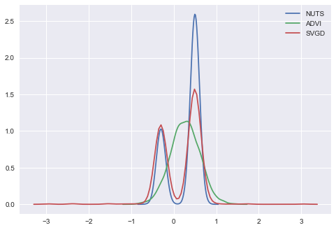
Looks much better. We have multimodal approximation with SVGD. Now it is possible to do arbitrary things with this variational approximation. For example we can create the same things as in the first model: \(x^2\) and \(sin(x)\)
In [29]:
# recall x ~ NormalMixture
a = x**2
b = pm.math.sin(x)
Replacements
To apply approximation to an arbitrary expression you should use
approx.apply_replacements or approx.sample_node methods
In [30]:
help(svgd_approx.apply_replacements)
Help on method apply_replacements in module pymc3.variational.opvi:

apply_replacements(node, deterministic=False, include=None, exclude=None, more_replacements=None) method of pymc3.variational.approximations.Empirical instance
    Replace variables in graph with variational approximation. By default, replaces all variables

    Parameters
    ----------
    node : Theano Variables (or Theano expressions)
        node or nodes for replacements
    deterministic : bool
        whether to use zeros as initial distribution
        if True - zero initial point will produce constant latent variables
    include : `list`
        latent variables to be replaced
    exclude : `list`
        latent variables to be excluded for replacements
    more_replacements : `dict`
        add custom replacements to graph, e.g. change input source

    Returns
    -------
    node(s) with replacements
basic usage
In [31]:
a_sample = svgd_approx.apply_replacements(a)
In [32]:
a_sample.eval()
Out[32]:
array(0.12294609099626541, dtype=float32)
In [33]:
a_sample.eval()
Out[33]:
array(0.08086667209863663, dtype=float32)
In [34]:
a_sample.eval()
Out[34]:
array(0.047388263046741486, dtype=float32)
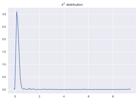
Every time we get different value for the same theano node. That is because it is stochastic. After replacements we are free and do not depend on pymc3 model. We now depend on approximation. Changing it will change the distribution for stochastic nodes
In [35]:
sns.kdeplot(np.array([a_sample.eval() for _ in range(2000)]));
plt.title('$x^2$ distribution');
There is a more convinient way to get lots of samples at once:
sample_node
In [36]:
a_samples = svgd_approx.sample_node(a, size=1000)
In [37]:
sns.kdeplot(a_samples.eval());
plt.title('$x^2$ distribution');
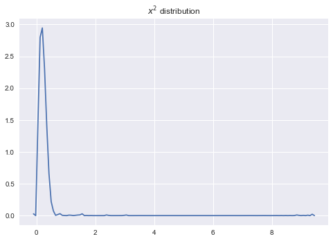
We get approximately the same picture
In [38]:
a_samples.eval().shape
Out[38]:
(1000,)
In [39]:
a_sample.eval().shape
Out[39]:
()
In sample_node function additional dimension is added in the first
position. So taking expectations, calculating variance is done by
axis=0
In [40]:
a_samples.var(0).eval() # variance
Out[40]:
array(0.14864803850650787, dtype=float32)
In [41]:
a_samples.mean(0).eval() # mean
Out[41]:
array(0.2578691840171814, dtype=float32)
Symbolic sample size is OK too
In [44]:
i = theano.tensor.iscalar('i')
i.tag.test_value = 1
a_samples_i = svgd_approx.sample_node(a, size=i)
In [45]:
a_samples_i.eval({i: 100}).shape
Out[45]:
(100,)
In [46]:
a_samples_i.eval({i: 10000}).shape
Out[46]:
(10000,)
But unfortunately only scalar size is supported.
converting trace to Approximation
There is a neat feature to convert any trace to Approximation. It will
have the same API as approximations above with same
apply_replacemets/sample_node methods
In [47]:
trace_approx = pm.Empirical(trace, model=model)
In [48]:
trace_approx
Out[48]:
<pymc3.variational.approximations.Empirical at 0x121bc4eb8>
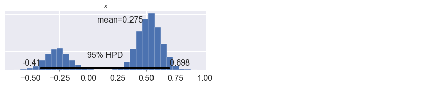
In [49]:
pm.plot_posterior(trace_approx.sample(10000));
Multilabel logistic regression
Favorite Iris dataset. One of the best illustrative example for using
Tracker can be done with Iris. We’ll do multilabel classification
there and compute expected accuracy score.
In [50]:
# First of all
from sklearn.datasets import load_iris
from sklearn.model_selection import train_test_split
import theano.tensor as tt
import pandas as pd
X, y = load_iris(True)
X_train, X_test, y_train, y_test = train_test_split(X, y)

Complex model for this illustratice example is is not needed as data classes are roughly linearly separable. Thus we are going to fit multinomial logistic regression.
In [51]:
Xt = theano.shared(X_train)
yt = theano.shared(y_train)
with pm.Model() as model:
    β = pm.Normal('β', 0, 1e2, shape=(4, 3))
    a = pm.Flat('a', shape=(3,))
    z = tt.nnet.softmax(Xt.dot(β) + a)
    observed = pm.Categorical('obs', p=z, observed=yt)
Applying replacements in practice
Models defined with pymc3 have symbolic inputs for latent variables. To
evaluate an espression that requires knoledge about latents one needs to
pass values for latent variables. In VI setup we have an approximation
for these variables ant it happens to be very usefull in practice.
Having a simple functions that removes all symbolic dependencies is
valuable. These functions are sample_node and apply_replacements
described above. Before we did not use the full power of replacements.
There is a usefull shortcut for applying even more replacements at once.
To get accuracy under approximate posterior we need to use
apply_replacements or sample_node. It’s better to get the whole
distribution at each step to draw neat plot so sample_node is our
choice. As mentioned above we can apply more replacements in single
function call. It can be done with readable kwarg more_replacements
in both replacement functions.
HINT: You can use more_replacements argument when calling
fit too
pm.fit(more_replacements={full_data: minibatch_data})inference.fit(more_replacements={full_data: minibatch_data})
In [52]:
with model:
    # We'll use SVGD
    inference = pm.SVGD(n_particles=500, jitter=1)
    # shortcut reference to approximation
    approx = inference.approx
    # Here we need `more_replacements` to change train_set to test_set
    test_probs = approx.sample_node(z, more_replacements={
        Xt: X_test
    })
    # For train set no more replacements needed
    train_probs = approx.sample_node(z)
    # Now we have 100 sampled probabilities (default argument) for each observation
Next we create symbolic expressions for sampled accuracy scores
In [53]:
test_ok = tt.eq(test_probs.argmax(-1), y_test)
train_ok = tt.eq(train_probs.argmax(-1), y_train)
test_accuracy = test_ok.mean(-1)
train_accuracy = train_ok.mean(-1)
Tracker expects callables so we can pass .eval method of theano node
that is function itself. Call to this function is cached and will be
reused.
In [54]:
eval_tracker = pm.callbacks.Tracker(
    test_accuracy=test_accuracy.eval,
    train_accuracy=train_accuracy.eval
)
In [55]:
inference.fit(
    100,
    callbacks=[eval_tracker]
)
100%|██████████| 100/100 [00:08<00:00, 12.50it/s]
Out[55]:
<pymc3.variational.approximations.Empirical at 0x1226bda20>
In [56]:
import seaborn as sns
sns.tsplot(np.asarray(eval_tracker['test_accuracy']).T, color='red')
sns.tsplot(np.asarray(eval_tracker['train_accuracy']).T, color='blue')
plt.legend(['test_accuracy', 'train_accuracy'])
plt.title('Training Progress')
Out[56]:
<matplotlib.text.Text at 0x123176be0>
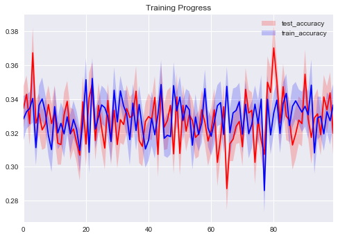
We have no training progress here. We are likely to change optimization method and increase learning rate.
In [57]:
inference.fit(
    400, obj_optimizer=pm.sgd(learning_rate=0.1),
    callbacks=[eval_tracker]
);
100%|██████████| 400/400 [00:27<00:00, 14.39it/s]
In [58]:
sns.tsplot(np.asarray(eval_tracker['test_accuracy']).T, color='red', alpha=.5)
sns.tsplot(np.asarray(eval_tracker['train_accuracy']).T, color='blue', alpha=.5)
plt.legend(['test_accuracy', 'train_accuracy'])
plt.title('Training Progress');
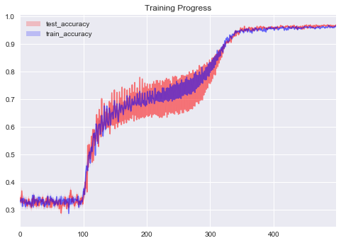
Much better. With Tracker we were able to track our progress and
choose good training schedule
Minibatches
Another usefull feature is Minibatch training. When your data is too
large there is no reason to use full dataset to compute gradients. There
is a nice API in pymc3 to handle these cases. You can reference
pm.Minibatch for details
In [59]:
# easy workflow like with regular tensor
issubclass(pm.Minibatch, theano.tensor.TensorVariable)
Out[59]:
True
Data
In [60]:
data = np.random.rand(400000, 100)    # initial
data *= np.random.randint(1, 10, size=(100,))# our std
data += np.random.rand(100) * 10    # our mean
no minibatch inference
In [61]:
with pm.Model() as model:
    mu = pm.Flat('mu', shape=(100,))
    sd = pm.HalfNormal('sd', shape=(100,))
    lik = pm.Normal('lik', mu, sd, observed=data)
One can create a custom special purpose callback. Here we define hard stop callback that helps stopping very slow inference not by hand but after concrete iteration. Signature is pretty simple
In [62]:
def stop_after_10(approx, loss_history, i):
    if (i > 0) and (i % 10) == 0:
        raise StopIteration('I was slow, sorry')
In [63]:
with model:
    advifit = pm.fit(callbacks=[stop_after_10])
Average Loss = 6.0648e+09:   0%|          | 10/10000 [00:22<6:03:15,  2.18s/it]
I was slow, sorry
Interrupted at 10 [0%]: Average Loss = 6.5297e+09
Inference is too slow, 2.18 seconds per iteration :(
minibatch inference
In [64]:
X = pm.Minibatch(data, batch_size=500)

with pm.Model() as model:
    mu = pm.Flat('mu', shape=(100,))
    sd = pm.HalfNormal('sd', shape=(100,))
    lik = pm.Normal('lik', mu, sd, observed=X, total_size=data.shape)
In [65]:
with model:
    advifit = pm.fit()
Average Loss = 1.2496e+08: 100%|██████████| 10000/10000 [00:11<00:00, 870.31it/s]
Finished [100%]: Average Loss = 1.2489e+08
In [66]:
plt.plot(advifit.hist);
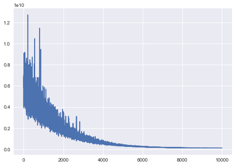
Minibatch inference is drasticaly faster. Full documentation for minibatch can be accessed via docstring. Multidimensional minibatches may be needed for some corner cases where you do matrix factorization or model is very wide.
In [67]:
print(pm.Minibatch.__doc__)
Multidimensional minibatch that is pure TensorVariable

    Parameters
    ----------
    data : :class:`ndarray`
        initial data
    batch_size : `int` or `List[int|tuple(size, random_seed)]`
        batch size for inference, random seed is needed
        for child random generators
    dtype : `str`
        cast data to specific type
    broadcastable : tuple[bool]
        change broadcastable pattern that defaults to `(False, ) * ndim`
    name : `str`
        name for tensor, defaults to "Minibatch"
    random_seed : `int`
        random seed that is used by default
    update_shared_f : `callable`
        returns :class:`ndarray` that will be carefully
        stored to underlying shared variable
        you can use it to change source of
        minibatches programmatically
    in_memory_size : `int` or `List[int|slice|Ellipsis]`
        data size for storing in theano.shared

    Attributes
    ----------
    shared : shared tensor
        Used for storing data
    minibatch : minibatch tensor
        Used for training

    Examples
    --------
    Consider we have data
    >>> data = np.random.rand(100, 100)

    if we want 1d slice of size 10 we do
    >>> x = Minibatch(data, batch_size=10)

    Note, that your data is cast to `floatX` if it is not integer type
    But you still can add `dtype` kwarg for :class:`Minibatch`

    in case we want 10 sampled rows and columns
    `[(size, seed), (size, seed)]` it is
    >>> x = Minibatch(data, batch_size=[(10, 42), (10, 42)], dtype='int32')
    >>> assert str(x.dtype) == 'int32'

    or simpler with default random seed = 42
    `[size, size]`
    >>> x = Minibatch(data, batch_size=[10, 10])

    x is a regular :class:`TensorVariable` that supports any math
    >>> assert x.eval().shape == (10, 10)

    You can pass it to your desired model
    >>> with pm.Model() as model:
    ...     mu = pm.Flat('mu')
    ...     sd = pm.HalfNormal('sd')
    ...     lik = pm.Normal('lik', mu, sd, observed=x, total_size=(100, 100))

    Then you can perform regular Variational Inference out of the box
    >>> with model:
    ...     approx = pm.fit()

    Notable thing is that :class:`Minibatch` has `shared`, `minibatch`, attributes
    you can call later
    >>> x.set_value(np.random.laplace(size=(100, 100)))

    and minibatches will be then from new storage
    it directly affects `x.shared`.
    the same thing would be but less convenient
    >>> x.shared.set_value(pm.floatX(np.random.laplace(size=(100, 100))))

    programmatic way to change storage is as follows
    I import `partial` for simplicity
    >>> from functools import partial
    >>> datagen = partial(np.random.laplace, size=(100, 100))
    >>> x = Minibatch(datagen(), batch_size=10, update_shared_f=datagen)
    >>> x.update_shared()

    To be more concrete about how we get minibatch, here is a demo
    1) create shared variable
    >>> shared = theano.shared(data)

    2) create random slice of size 10
    >>> ridx = pm.tt_rng().uniform(size=(10,), low=0, high=data.shape[0]-1e-10).astype('int64')

    3) take that slice
    >>> minibatch = shared[ridx]

    That's done. Next you can use this minibatch somewhere else.
    You can see that implementation does not require fixed shape
    for shared variable. Feel free to use that if needed.

    Suppose you need some replacements in the graph, e.g. change minibatch to testdata
    >>> node = x ** 2  # arbitrary expressions on minibatch `x`
    >>> testdata = pm.floatX(np.random.laplace(size=(1000, 10)))

    Then you should create a dict with replacements
    >>> replacements = {x: testdata}
    >>> rnode = theano.clone(node, replacements)
    >>> assert (testdata ** 2 == rnode.eval()).all()

    To replace minibatch with it's shared variable you should do
    the same things. Minibatch variable is accessible as an attribute
    as well as shared, associated with minibatch
    >>> replacements = {x.minibatch: x.shared}
    >>> rnode = theano.clone(node, replacements)

    For more complex slices some more code is needed that can seem not so clear
    >>> moredata = np.random.rand(10, 20, 30, 40, 50)

    default `total_size` that can be passed to `PyMC3` random node
    is then `(10, 20, 30, 40, 50)` but can be less verbose in some cases

    1) Advanced indexing, `total_size = (10, Ellipsis, 50)`
    >>> x = Minibatch(moredata, [2, Ellipsis, 10])

    We take slice only for the first and last dimension
    >>> assert x.eval().shape == (2, 20, 30, 40, 10)

    2) Skipping particular dimension, `total_size = (10, None, 30)`
    >>> x = Minibatch(moredata, [2, None, 20])
    >>> assert x.eval().shape == (2, 20, 20, 40, 50)

    3) Mixing that all, `total_size = (10, None, 30, Ellipsis, 50)`
    >>> x = Minibatch(moredata, [2, None, 20, Ellipsis, 10])
    >>> assert x.eval().shape == (2, 20, 20, 40, 10)