LKJ Prior for fitting a Multivariate Normal Model
Author: Austin Rochford
Outside of the
beta-binomial
model, the multivariate normal model is likely the most studied Bayesian
model in history. PyMC3 supports sampling from the LKJ
distribution.
The LKJ distribution represents the distribution on correlation matrices
and is conjugate to the multivariate normal distribution. This post will
show how to fit a simple multivariate normal model using pymc3 with
a normal-LKJ prior.
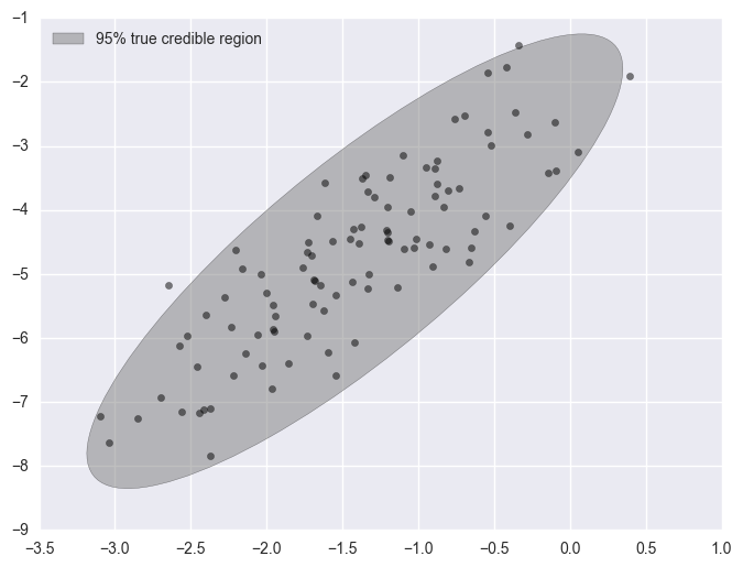
First, we generate some two-dimensional sample data.
In [1]:
%matplotlib inline
In [2]:
from matplotlib.patches import Ellipse
from matplotlib import pyplot as plt
import numpy as np
import pymc3 as pm
import scipy as sp
import seaborn as sns
from theano import tensor as tt
In [3]:
np.random.seed(3264602) # from random.org
In [4]:
N = 100

mu_actual = sp.stats.uniform.rvs(-5, 10, size=2)

cov_actual_sqrt = sp.stats.uniform.rvs(0, 2, size=(2, 2))
cov_actual = np.dot(cov_actual_sqrt.T, cov_actual_sqrt)

x = sp.stats.multivariate_normal.rvs(mu_actual, cov_actual, size=N)
In [5]:
var, U = np.linalg.eig(cov_actual)
angle = 180. / np.pi * np.arccos(np.abs(U[0, 0]))
In [6]:
fig, ax = plt.subplots(figsize=(8, 6))

blue = sns.color_palette()[0]

e = Ellipse(mu_actual, 2 * np.sqrt(5.991 * var[0]), 2 * np.sqrt(5.991 * var[1]), angle=-angle)
e.set_alpha(0.5)
e.set_facecolor('gray')
e.set_zorder(10);
ax.add_artist(e);

ax.scatter(x[:, 0], x[:, 1], c='k', alpha=0.5, zorder=11);

rect = plt.Rectangle((0, 0), 1, 1, fc='gray', alpha=0.5)
ax.legend([rect], ['95% true credible region'], loc=2);
The sampling distribution for our model is \(x_i \sim N(\mu, \Lambda)\), where \(\Lambda\) is the precision matrix of the distribution. The precision matrix is the inverse of the covariance matrix. The support of the LKJ distribution is the set of correlation matrices, not covariance matrices. We will use the separation strategy from Barnard et al. to combine an LKJ prior on the correlation matrix with a prior on the standard deviations of each dimension to produce a prior on the covariance matrix.
Let \(\sigma\) be the vector of standard deviations of each component of our normal distribution, and \(\mathbf{C}\) be the correlation matrix. The relationship
shows that priors on \(\sigma\) and \(\mathbf{C}\) will induce a prior on \(\Sigma\). Following Barnard et al., we place a standard lognormal prior each the elements \(\sigma\), and an LKJ prior on the correlation matric \(\mathbf{C}\). The LKJ distribution requires a shape parameter \(\nu > 0\). If \(\mathbf{C} \sim LKJ(\nu)\), then \(f(\mathbf{C}) \propto |\mathbf{C}|^{\nu - 1}\) (here \(|\cdot|\) is the determinant).
We can now begin to build this model in pymc3. As you can see, we
are passing summary statistics to testval which will be used as the
starting point when we do inference further below. When summary
statistics are available, it is always a good idea to use them in this
manner.
In [7]:
init_sigma = np.std(x, axis=0)
init_corr = np.corrcoef(x, rowvar=0)[0, 1]
with pm.Model() as model:
    sigma = pm.Lognormal('sigma', np.zeros(2), np.ones(2), shape=2, testval=init_sigma)

    nu = pm.Uniform('nu', 0, 5)
    C_triu = pm.LKJCorr('C_triu', nu, 2, testval=init_corr)
There is a slight complication in pymc3‘s handling of the
LKJCorr distribution; pymc3 represents the support of this
distribution as a one-dimensional vector of the upper triangular
elements of the full covariance matrix.
In [8]:
C_triu.tag.test_value.shape
Out[8]:
(1,)
In order to build a the full correlation matric \(\mathbf{C}\), we
first build a \(2 \times 2\) tensor whose values are all C_triu
and then set the diagonal entries to one. (Recall that a correlation
matrix must be symmetric and positive definite with all diagonal entries
equal to one.) We can then proceed to build the covariance matrix
\(\Sigma\) and the precision matrix \(\Lambda\).
In [9]:
with model:
    C = pm.Deterministic('C', tt.fill_diagonal(C_triu[np.zeros((2, 2), dtype=np.int64)], 1.))

    sigma_diag = pm.Deterministic('sigma_mat', tt.nlinalg.diag(sigma))
    cov = pm.Deterministic('cov', tt.nlinalg.matrix_dot(sigma_diag, C, sigma_diag))
In [10]:
cov.tag.test_value
Out[10]:
array([[ 0.54737873,  0.88092866],
       [ 0.88092866,  1.98234664]])
While defining C in terms of C_triu was simple in this case
because our sampling distribution is two-dimensional, the example from
this StackOverflow
question
shows how to generalize this transformation to arbitrarily many
dimensions.
Finally, we define the prior on \(\mu\) and the sampling distribution.
In [11]:
with model:
    mu = pm.MvNormal('mu', 0, cov, shape=2, testval=np.mean(x, axis=0))

    x_ = pm.MvNormal('x', mu, cov, observed=x)
We are now ready to fit this model using pymc3.
In [12]:
n_samples = 4000
In [13]:
with model:
    trace_ = pm.sample(n_samples, pm.Metropolis())
100%|██████████| 4000/4000 [00:05<00:00, 718.12it/s]
In [14]:
trace = trace_[50:]
We see that the posterior estimate of \(\mu\) is reasonably accurate.
In [15]:
pm.traceplot(trace, varnames=['mu']);
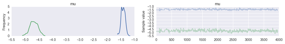
In [16]:
mu_actual
Out[16]:
array([-1.41866859, -4.8018335 ])
The estimates of the standard deviations are certainly biased.
In [17]:
pm.traceplot(trace, varnames=['sigma']);
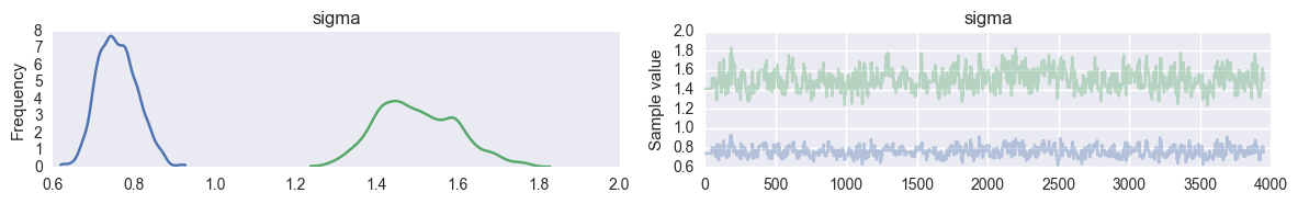
In [18]:
trace['sigma'].mean(axis=0)
Out[18]:
array([ 0.75945843, 1.50000803])
In [19]:
np.sqrt(var)
Out[19]:
array([ 0.3522422 , 1.58192855])
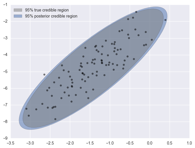
However, the 95% posterior credible region is visually quite close to the true credible region, so we can be fairly satisfied with our model.
In [20]:
post_cov = trace['cov'].mean(axis=0)

post_sigma, post_U = np.linalg.eig(post_cov)
post_angle = 180. / np.pi * np.arccos(np.abs(post_U[0, 0]))
In [21]:
fig, ax = plt.subplots(figsize=(8, 6))

blue = sns.color_palette()[0]

e = Ellipse(mu_actual, 2 * np.sqrt(5.991 * post_sigma[0]), 2 * np.sqrt(5.991 * post_sigma[1]), angle=-post_angle)
e.set_alpha(0.5)
e.set_facecolor(blue)
e.set_zorder(9);
ax.add_artist(e);

e = Ellipse(mu_actual, 2 * np.sqrt(5.991 * var[0]), 2 * np.sqrt(5.991 * var[1]), angle=-angle)
e.set_alpha(0.5)
e.set_facecolor('gray')
e.set_zorder(10);
ax.add_artist(e);

ax.scatter(x[:, 0], x[:, 1], c='k', alpha=0.5, zorder=11);

rect = plt.Rectangle((0, 0), 1, 1, fc='gray', alpha=0.5)
post_rect = plt.Rectangle((0, 0), 1, 1, fc=blue, alpha=0.5)
ax.legend([rect, post_rect],
          ['95% true credible region',
           '95% posterior credible region'],
          loc=2);